Take-home Exercise 3: Geographically Weighted Predictive Models: Rental price prediction based on location based data

Analysis

spdep

tmap

tidyverse

GWmodel

SpatialML

rsample

Metrics

olsrr

Author

Brian Lim

Published

October 27, 2024

Modified

November 3, 2024

3.1 Overview

In this take-home exercise, I will focus on prototyping a Geographically Weighted Predictive Model for my group’s Shiny App. This model allows users to input specific values for key variables and obtain rental price predictions for HDB flats in Singapore. The model considers variables such as flat type, proximity to kindergartens and MRT stations, the number of childcare centers within 500 meters, and distance to amenities like hawker centers, shopping malls, primary schools, and the CBD. By capturing these localized effects, the predictive model provides a user-friendly, data-driven tool for estimating monthly rent based on a flat’s characteristics and surrounding environment. The data preparation and Exploratory Data Analysis were handled by my groupmate, so for this exercise, I will load the data directly from an RDS file. For this exercise, I will load the prepared dataset directly from an RDS file for efficient model testing.

3.2 Getting Started

For this exercise, the following R packages will be used:

sf for handling geospatial data.
spdep for spatial dependence analysis, including computing spatial weights and conducting spatial autocorrelation tests such as Moran’s I and Geary’s C
tmap, a package for creating high-quality static and interactive maps, leveraging the Leaflet API for interactive visualizations.
tidyverse for performing data science tasks such as importing, wrangling and visualising data.
GWmodel provides techniques from a particular branch of spatial statistics,termed geographically-weighted (GW) models. GW models suit situations when data are not described well by some global model, but where there are spatial regions where a suitably localised calibration provides a better description.
SpatialML for a geographically weighted random forest regression including a function to find the optical bandwidth.
rsample to create and summarize different types of resampling objects.
Metrics implements metrics for regression, time series, binary classification, classification, and information retrieval problems.
olsrr provides tools for building OLS regression models using R

As readr, tidyr and dplyr are part of tidyverse package. The code chunk below will suffice to install and load the required packages in RStudio.

To install and load these packages into the R environment, we use the p_load function from the pacman package:

pacman::p_load(sf, spdep, tmap, tidyverse, GWmodel, SpatialML, rsample, Metrics, olsrr)

3.3 Importing Data into R

We will first import the rental dataset prepared by one of my teammates. Please refer to here for the details of the data wrangling.

rental.sf => contains the rental data from Jan 2020 to Sept 2024, as well as other fields like:
- Dependent:
  - Monthly Rental fee: monthly_rent
- Continuous:
  - Proximity measure: kindergarten, childcare, hawker, bus stops, shopping mall, mrt, primary schools, cbd
  - Count of amenities within specific distance: kindergarten, childcare, hawker, bus stops, shopping mall,
- Categorical:
  - Flat Type: flat_type
  - Town: town
  - Region: region

rental_sf <- read_rds("data/rds/rental_sf.rds")

Primarily, we will be working with numerical values to determine the variable correlations they have with monthly_rent. Based on the summary results below, we will first focus on the following columns:

1. no_of_kindergarten_500m

2. prox_kindergarten

3. no_of_childcare_500m

4. prox_childcare

5. no_of_hawker_500m

6. prox_hawker

7. no_of_busstop_500m

8. prox_busstop

9. no_of_shoppingmall_1km

10. prox_shoppingmall

11. prox_mrt

12. prox_prisch

13. prox_cbd

summary(rental_sf)

 rent_approval_date       town            flat_type          monthly_rent 
 Min.   :2024-01-01   Length:25713       Length:25713       Min.   : 500  
 1st Qu.:2024-03-01   Class :character   Class :character   1st Qu.:2700  
 Median :2024-05-01   Mode  :character   Mode  :character   Median :3100  
 Mean   :2024-04-29                                         Mean   :3102  
 3rd Qu.:2024-07-01                                         3rd Qu.:3500  
 Max.   :2024-09-01                                         Max.   :6500  
          geometry        region          no_of_kindergarten_500m
 POINT        :25713   Length:25713       Min.   : 0.000         
 epsg:3414    :    0   Class :character   1st Qu.: 1.000         
 +proj=tmer...:    0   Mode  :character   Median : 2.000         
                                          Mean   : 1.912         
                                          3rd Qu.: 3.000         
                                          Max.   :11.000         
 prox_kindergarten no_of_childcare_500m prox_childcare    no_of_hawker_500m
 Min.   :   0.0    Min.   : 0.000       Min.   :   0.00   Min.   :0.0000   
 1st Qu.: 171.7    1st Qu.: 6.000       1st Qu.:  71.08   1st Qu.:0.0000   
 Median : 272.0    Median : 8.000       Median : 117.53   Median :0.0000   
 Mean   : 296.6    Mean   : 8.495       Mean   : 126.71   Mean   :0.6711   
 3rd Qu.: 390.5    3rd Qu.:10.000       3rd Qu.: 170.96   3rd Qu.:1.0000   
 Max.   :3196.7    Max.   :28.000       Max.   :2952.48   Max.   :5.0000   
  prox_hawker       no_of_busstop_500m  prox_busstop    no_of_shoppingmall_1km
 Min.   :   6.981   Min.   : 3.00      Min.   : 15.43   Min.   : 0.00         
 1st Qu.: 301.816   1st Qu.:12.00      1st Qu.: 73.62   1st Qu.: 1.00         
 Median : 530.754   Median :15.00      Median :107.18   Median : 2.00         
 Mean   : 672.403   Mean   :15.28      Mean   :114.66   Mean   : 1.78         
 3rd Qu.: 907.293   3rd Qu.:18.00      3rd Qu.:145.81   3rd Qu.: 3.00         
 Max.   :2867.630   Max.   :32.00      Max.   :391.47   Max.   :16.00         
 prox_shoppingmall    prox_mrt         prox_prisch        prox_cbd    
 Min.   :   0.0    Min.   :   9.112   Min.   :   0.0   Min.   :  722  
 1st Qu.: 388.7    1st Qu.: 250.080   1st Qu.: 249.3   1st Qu.: 7412  
 Median : 617.7    Median : 423.233   Median : 385.4   Median :11340  
 Mean   : 689.8    Mean   : 495.644   Mean   : 443.9   Mean   :10956  
 3rd Qu.: 920.1    3rd Qu.: 666.385   3rd Qu.: 557.4   3rd Qu.:14314  
 Max.   :3222.7    Max.   :3446.893   Max.   :3293.3   Max.   :19758

The entire data are split into training and test data sets with 65% and 35% respectively by using initial_split() of rsample package.

set.seed(1234)
rental_split <- initial_split(rental_sf, 
                              prop = 6.5/10,)
train_data <- training(rental_split)
test_data <- testing(rental_split)

write_rds(train_data, "data/rds/model/train_data.rds")
write_rds(test_data, "data/rds/model/test_data.rds")

train_data <- read_rds("data/rds/model/train_data.rds")
test_data <- read_rds("data/rds/model/test_data.rds")

rental_nogeo <- rental_sf %>%
  select(7:19) %>%
  st_drop_geometry()

As we are more interested in predicting rental prices of property based on different locations across Singpaore, we will start by examining the only numeric independent values of the rental.sf data frame

names(rental_nogeo)

 [1] "no_of_kindergarten_500m" "prox_kindergarten"      
 [3] "no_of_childcare_500m"    "prox_childcare"         
 [5] "no_of_hawker_500m"       "prox_hawker"            
 [7] "no_of_busstop_500m"      "prox_busstop"           
 [9] "no_of_shoppingmall_1km"  "prox_shoppingmall"      
[11] "prox_mrt"                "prox_prisch"            
[13] "prox_cbd"

3.4 Computing Correlation Matrix

Before loading the predictors into a predictive model, it is always a good practice to use correlation matrix to examine if there is sign of multicolinearity.

The code chunk below is used to plot a scatterplot matrix of the relationship between the independent variables in rental.sf data.frame.

corrplot::corrplot(cor(rental_nogeo), 
                   diag = FALSE, 
                   order = "AOE",
                   tl.pos = "td", 
                   tl.cex = 0.5, 
                   method = "number", 
                   type = "upper")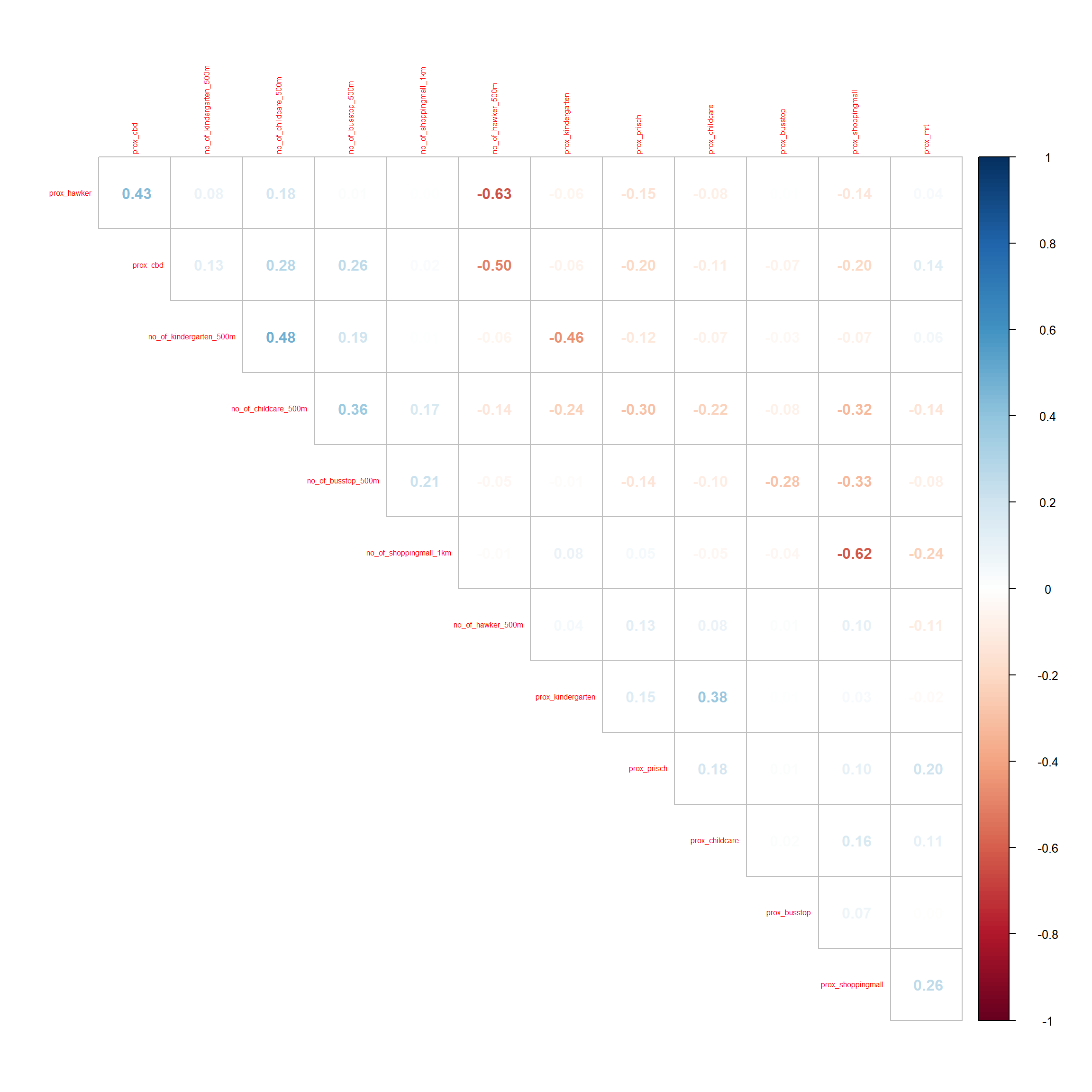

After viewing the various correlation matrices above, all the correlation values are below 0.8. Hence, there is no sign of multicolinearity.

3.5 Building a non-spatial multiple linear regression

We will now go about building a non-spatial multi-linear regression. Given that flat_type is categorical and has been shown to significantly impact rental prices, it’s appropriate to retain it. Variables like flat_type have proven theoretical and empirical justification for their inclusion based on their substantial effect on monthly rental price.

train_data <- read_rds("data/rds/model/train_data.rds")
test_data <- read_rds("data/rds/model/test_data.rds")

Show the code

rental_price_mlr <- lm(monthly_rent ~ 
                  flat_type + no_of_kindergarten_500m + prox_kindergarten +
                  no_of_childcare_500m + no_of_hawker_500m + prox_childcare +
                  prox_hawker + no_of_busstop_500m + prox_busstop + 
                  no_of_shoppingmall_1km + prox_shoppingmall +
                  prox_mrt + prox_prisch +
                  prox_cbd,
                data=train_data)

summary(rental_price_mlr)


Call:
lm(formula = monthly_rent ~ flat_type + no_of_kindergarten_500m + 
    prox_kindergarten + no_of_childcare_500m + no_of_hawker_500m + 
    prox_childcare + prox_hawker + no_of_busstop_500m + prox_busstop + 
    no_of_shoppingmall_1km + prox_shoppingmall + prox_mrt + prox_prisch + 
    prox_cbd, data = train_data)

Residuals:
     Min       1Q   Median       3Q      Max 
-3062.83  -286.72    65.87   348.22  2720.83 

Coefficients:
                          Estimate Std. Error t value Pr(>|t|)    
(Intercept)              3.229e+03  3.497e+01  92.323  < 2e-16 ***
flat_type4-ROOM          6.540e+02  1.026e+01  63.763  < 2e-16 ***
flat_type5-ROOM          9.203e+02  1.195e+01  77.030  < 2e-16 ***
no_of_kindergarten_500m  8.559e+00  3.788e+00   2.260  0.02385 *  
prox_kindergarten       -8.094e-02  2.959e-02  -2.735  0.00624 ** 
no_of_childcare_500m    -7.138e+00  1.541e+00  -4.633 3.64e-06 ***
no_of_hawker_500m       -8.987e-01  6.881e+00  -0.131  0.89609    
prox_childcare          -2.000e-02  5.015e-02  -0.399  0.69011    
prox_hawker             -6.219e-02  1.140e-02  -5.457 4.92e-08 ***
no_of_busstop_500m       9.605e-01  1.110e+00   0.866  0.38677    
prox_busstop             7.130e-02  7.997e-02   0.892  0.37263    
no_of_shoppingmall_1km  -2.101e+00  3.687e+00  -0.570  0.56886    
prox_shoppingmall       -8.636e-02  1.476e-02  -5.849 5.03e-09 ***
prox_mrt                -1.063e-01  1.391e-02  -7.642 2.25e-14 ***
prox_prisch              4.032e-02  1.674e-02   2.408  0.01606 *  
prox_cbd                -3.886e-02  1.179e-03 -32.962  < 2e-16 ***
---
Signif. codes:  0 '***' 0.001 '**' 0.01 '*' 0.05 '.' 0.1 ' ' 1

Residual standard error: 547.7 on 16697 degrees of freedom
Multiple R-squared:  0.3144,    Adjusted R-squared:  0.3137 
F-statistic: 510.3 on 15 and 16697 DF,  p-value: < 2.2e-16

Based on the coefficient section, we can see that not all the independent variables are statistically significant, and some variables can be removed from our model based on their p-value field (Pr > 0.05).

The following variables should be removed from the model due to their high p-values, indicating they are not statisitically significant predictors of monthly rent:

1. no_of_hawker_500m (p = 0.89609)

2. prox_childcare (p = 0.69011)

3. no_of_busstop_500m (p = 0.38677)

4. prox_busstop (p = 0.37263)

5. no_of_shoppingmall_1km (p = 0.56886)

Now we will update the model by removing the 5 variables

Show the code

rental_price_mlr <- lm(formula = monthly_rent ~ flat_type + no_of_kindergarten_500m + prox_kindergarten +
                  no_of_childcare_500m + prox_hawker + prox_shoppingmall +
                  prox_mrt + prox_prisch + prox_cbd, 
                 data = train_data)

# Display the publication-quality table
ols_regress(rental_price_mlr)

                           Model Summary                             
--------------------------------------------------------------------
R                         0.561       RMSE                  547.483 
R-Squared                 0.314       MSE                299935.128 
Adj. R-Squared            0.314       Coef. Var              17.672 
Pred R-Squared            0.313       AIC                258215.452 
MAE                     412.938       SBC                258308.139 
--------------------------------------------------------------------
 RMSE: Root Mean Square Error 
 MSE: Mean Square Error 
 MAE: Mean Absolute Error 
 AIC: Akaike Information Criteria 
 SBC: Schwarz Bayesian Criteria 

                                     ANOVA                                       
--------------------------------------------------------------------------------
                      Sum of                                                    
                     Squares           DF      Mean Square       F         Sig. 
--------------------------------------------------------------------------------
Regression    2295968877.016           10    229596887.702    765.488    0.0000 
Residual      5009516507.263        16702       299935.128                      
Total         7305485384.279        16712                                       
--------------------------------------------------------------------------------

                                            Parameter Estimates                                             
-----------------------------------------------------------------------------------------------------------
                  model        Beta    Std. Error    Std. Beta       t        Sig        lower       upper 
-----------------------------------------------------------------------------------------------------------
            (Intercept)    3240.088        23.849                 135.858    0.000    3193.341    3286.834 
        flat_type4-ROOM     654.702        10.195        0.484     64.215    0.000     634.718     674.686 
        flat_type5-ROOM     921.148        11.884        0.600     77.510    0.000     897.853     944.443 
no_of_kindergarten_500m       8.553         3.704        0.019      2.309    0.021       1.293      15.813 
      prox_kindergarten      -0.085         0.027       -0.023     -3.152    0.002      -0.138      -0.032 
   no_of_childcare_500m      -6.901         1.502       -0.038     -4.594    0.000      -9.845      -3.956 
            prox_hawker      -0.062         0.010       -0.047     -6.449    0.000      -0.081      -0.043 
      prox_shoppingmall      -0.084         0.012       -0.051     -7.117    0.000      -0.107      -0.061 
               prox_mrt      -0.106         0.014       -0.054     -7.699    0.000      -0.133      -0.079 
            prox_prisch       0.038         0.017        0.016      2.297    0.022       0.006       0.070 
               prox_cbd      -0.039         0.001       -0.269    -35.002    0.000      -0.041      -0.036 
-----------------------------------------------------------------------------------------------------------

Interpretation

Model Performance:
- The R-squared value is 0.314, indicating that about 31.4% of the variability in monthly rent is explained by the model. While it shows some predictive capability, other factors might still influence rental prices.
Key Predictors:
- Significant Variables: The predictors with low p-values (e.g., flat type, number of kindergartens, proximity to hawker centers, shopping malls, MRT stations, primary schools, and CBD) significantly influence monthly rent.
- Noteworthy Coefficients:
  - flat_type: Larger room types (4-ROOM, 5-ROOM) show substantial positive impacts on monthly rent.
  - prox_cbd: Rent decreases as distance from the CBD increases, with each unit increase in distance reducing the monthly rent by about 0.039.
Model Error and Diagnostics:
1. RMSE: 547.5, suggesting a reasonable prediction accuracy
2. MAE: 412.9, reflecting an average prediction error of about $413

3.6 Constructing the adaptive bandwidth gwr model

Now, we can go ahead to calibrate the gwr-based hedonic pricing model by using adaptive bandwidth and Gaussian kernel. First we use bw.gwr() of GWmodel package to determine the optimal bandwidth to be used

train_data_sp <- as_Spatial(train_data)
train_data_sp

class       : SpatialPointsDataFrame 
features    : 16713 
extent      : 11597.31, 45192.3, 28097.64, 48741.06  (xmin, xmax, ymin, ymax)
crs         : +proj=tmerc +lat_0=1.36666666666667 +lon_0=103.833333333333 +k=1 +x_0=28001.642 +y_0=38744.572 +ellps=WGS84 +towgs84=0,0,0,0,0,0,0 +units=m +no_defs 
variables   : 18
names       : rent_approval_date,       town, flat_type, monthly_rent,         region, no_of_kindergarten_500m,    prox_kindergarten, no_of_childcare_500m,       prox_childcare, no_of_hawker_500m,      prox_hawker, no_of_busstop_500m,     prox_busstop, no_of_shoppingmall_1km, prox_shoppingmall, ... 
min values  :              19723, ANG MO KIO,    3-ROOM,          500, CENTRAL REGION,                       0, 6.59828462646688e-05,                    0, 6.26024982260832e-06,                 0,  6.9808810867684,                  3, 15.4274594853233,                      0,                 0, ... 
max values  :              19967,     YISHUN,    5-ROOM,         6500,    WEST REGION,                      11,      3196.6660398211,                   28,     2952.47979062617,                 5, 2867.63031236184,                 32, 391.470766976464,                     16,  3222.67183763499, ...

Show the code

bw_adaptive <- bw.gwr(monthly_rent ~ 
                  flat_type + no_of_kindergarten_500m + prox_kindergarten +
                  no_of_childcare_500m + prox_hawker + prox_shoppingmall +
                  prox_mrt + prox_prisch + prox_cbd,
                  data=train_data_sp,
                  approach="CV",
                  kernel="gaussian",
                  adaptive=TRUE,
                  longlat=FALSE)

write_rds(bw_adaptive, "data/rds/model/bw_adaptive.rds")

bw_adaptive <- read_rds("data/rds/model/bw_adaptive.rds")
bw_adaptive

[1] 184

Inisghts

Optimal Bandwidth:

Here, the optimal adaptive bandwidth is found to be 184 (based on the lowest CV score of 4484696643).
This bandwidth indicates that for each local regression in the GWR model, the 184 nearest neighbors are included, providing a balance between capturing spatial variation and maintaining model stability.

After identifying the optimal adaptive bandwidth (bw_adaptive) for running a Geographically Weighted Regression (GWR) with cross-validation, we use this bw_adaptive value in the next step with gwr.basic will allow you to fit the GWR model itself.

In short, this step allows you to create a spatially-varying model, which helps identify how different factors contribute to monthly_rent differently across locations.

Now we can to calibrate the gwr-based hedonic pricing model using adaptive bandwidth and gaussian kernel.

Show the code

gwr_adaptive <- gwr.basic(formula = monthly_rent ~ 
                  flat_type + no_of_kindergarten_500m + prox_kindergarten +
                  no_of_childcare_500m + prox_hawker + prox_shoppingmall +
                  prox_mrt + prox_prisch + prox_cbd,
                  data=train_data_sp,
                          bw=bw_adaptive, 
                          kernel = 'gaussian', 
                          adaptive=TRUE,
                          longlat = FALSE)

write_rds(gwr_adaptive, "data/rds/model/gwr_adaptive.rds")

gwr_adaptive <- read_rds("data/rds/model/gwr_adaptive.rds")

This code produces the GWR model using the adaptive bandwidth previously calculated. Running this step is essential for performing the actual localized regression analysis and obtaining spatially varying coefficients, which will reveal how the influence of each predictor on rental prices varies across the area. This model will give you insights into spatial patterns in rental prices, helping you to understand which factors are most significant in different locations.

gwr_adaptive

   ***********************************************************************
   *                       Package   GWmodel                             *
   ***********************************************************************
   Program starts at: 2024-11-03 00:38:14.363774 
   Call:
   gwr.basic(formula = monthly_rent ~ flat_type + no_of_kindergarten_500m + 
    prox_kindergarten + no_of_childcare_500m + prox_hawker + 
    prox_shoppingmall + prox_mrt + prox_prisch + prox_cbd, data = train_data_sp, 
    bw = bw_adaptive, kernel = "gaussian", adaptive = TRUE, longlat = FALSE)

   Dependent (y) variable:  monthly_rent
   Independent variables:  flat_type no_of_kindergarten_500m prox_kindergarten no_of_childcare_500m prox_hawker prox_shoppingmall prox_mrt prox_prisch prox_cbd
   Number of data points: 16713
   ***********************************************************************
   *                    Results of Global Regression                     *
   ***********************************************************************

   Call:
    lm(formula = formula, data = data)

   Residuals:
     Min       1Q   Median       3Q      Max 
-3060.57  -286.94    66.18   348.38  2725.20 

   Coefficients:
                             Estimate Std. Error t value Pr(>|t|)    
   (Intercept)              3.240e+03  2.385e+01 135.858  < 2e-16 ***
   flat_type4-ROOM          6.547e+02  1.020e+01  64.215  < 2e-16 ***
   flat_type5-ROOM          9.211e+02  1.188e+01  77.510  < 2e-16 ***
   no_of_kindergarten_500m  8.553e+00  3.704e+00   2.309  0.02095 *  
   prox_kindergarten       -8.478e-02  2.690e-02  -3.152  0.00162 ** 
   no_of_childcare_500m    -6.901e+00  1.502e+00  -4.594 4.38e-06 ***
   prox_hawker             -6.226e-02  9.654e-03  -6.449 1.16e-10 ***
   prox_shoppingmall       -8.396e-02  1.180e-02  -7.117 1.15e-12 ***
   prox_mrt                -1.062e-01  1.379e-02  -7.699 1.45e-14 ***
   prox_prisch              3.800e-02  1.655e-02   2.297  0.02165 *  
   prox_cbd                -3.863e-02  1.104e-03 -35.002  < 2e-16 ***

   ---Significance stars
   Signif. codes:  0 '***' 0.001 '**' 0.01 '*' 0.05 '.' 0.1 ' ' 1 
   Residual standard error: 547.7 on 16702 degrees of freedom
   Multiple R-squared: 0.3143
   Adjusted R-squared: 0.3139 
   F-statistic: 765.5 on 10 and 16702 DF,  p-value: < 2.2e-16 
   ***Extra Diagnostic information
   Residual sum of squares: 5009516507
   Sigma(hat): 547.5158
   AIC:  258215.5
   AICc:  258215.5
   BIC:  241711.8
   ***********************************************************************
   *          Results of Geographically Weighted Regression              *
   ***********************************************************************

   *********************Model calibration information*********************
   Kernel function: gaussian 
   Adaptive bandwidth: 184 (number of nearest neighbours)
   Regression points: the same locations as observations are used.
   Distance metric: Euclidean distance metric is used.

   ****************Summary of GWR coefficient estimates:******************
                                  Min.     1st Qu.      Median     3rd Qu.
   Intercept               -4.1239e+03  2.2785e+03  2.9224e+03  3.3464e+03
   flat_type4.ROOM          1.5958e+02  4.7323e+02  5.8078e+02  7.1121e+02
   flat_type5.ROOM          3.3315e+02  7.3309e+02  8.7484e+02  1.0579e+03
   no_of_kindergarten_500m -4.4557e+02 -3.1163e+01 -3.5370e+00  1.3943e+01
   prox_kindergarten       -2.7091e+00 -1.9117e-01  2.9232e-02  2.1290e-01
   no_of_childcare_500m    -7.8560e+01 -6.0831e+00  2.5467e+00  1.1740e+01
   prox_hawker             -6.8246e-01 -1.0095e-01  3.7093e-02  2.0007e-01
   prox_shoppingmall       -1.3366e+00 -1.4787e-01 -5.2000e-02  5.9172e-02
   prox_mrt                -2.4673e+00 -3.2010e-01 -1.8481e-01 -6.2536e-02
   prox_prisch             -1.1783e+00 -1.1478e-01  1.6581e-02  1.1858e-01
   prox_cbd                -1.0204e+00 -6.5047e-02 -1.0502e-02  3.4669e-02
                                 Max.
   Intercept               10751.4755
   flat_type4.ROOM          1196.1883
   flat_type5.ROOM          1495.6959
   no_of_kindergarten_500m   112.0738
   prox_kindergarten           0.6535
   no_of_childcare_500m      107.6404
   prox_hawker                 1.5006
   prox_shoppingmall           1.4020
   prox_mrt                    0.7157
   prox_prisch                 1.2324
   prox_cbd                    0.9232
   ************************Diagnostic information*************************
   Number of data points: 16713 
   Effective number of parameters (2trace(S) - trace(S'S)): 585.6495 
   Effective degrees of freedom (n-2trace(S) + trace(S'S)): 16127.35 
   AICc (GWR book, Fotheringham, et al. 2002, p. 61, eq 2.33): 256327.1 
   AIC (GWR book, Fotheringham, et al. 2002,GWR p. 96, eq. 4.22): 255849.9 
   BIC (GWR book, Fotheringham, et al. 2002,GWR p. 61, eq. 2.34): 243063.8 
   Residual sum of squares: 4238886846 
   R-square value:  0.4197666 
   Adjusted R-square value:  0.3986946 

   ***********************************************************************
   Program stops at: 2024-11-03 00:39:34.720698

Insights

This analysis captures how each variable’s impact on rental prices varies across different spatial locations. Here’s a breakdown of the key results:

1. Global Regression Results

Significant variables (based on p-values < 0.05) include: - flat_type: Different flat types significantly impact rental prices. - Proximity to various facilities (e.g., prox_kindergarten, prox_hawker, prox_shoppingmall, prox_mrt, prox_cbd) also shows significant impact, with proximity to the Central Business District (prox_cbd) having a strong negative effect.

2. GWR Results

Adaptive Bandwidth: The optimal bandwidth is 184, determined via cross-validation. This bandwidth allows the model to capture spatially varying relationships, adjusting the number of nearest neighbors for each location.
prox_cbd has a median negative effect but varies across locations, indicating that distance to the CBD does not uniformly affect rental prices.
Insignificant Features: All of the features listed have p-values less than 0.05, indicating that they are statistically significant. However, if you’re looking for features that are less impactful:

prox_kindergarten: p = 0.00162
prox_prisch: p = 0.02165

R-squared: 0.4198, indicating that the GWR model explains around 41.98% of the variance in rental prices—an improvement over the global model.
AICc: 256327.1, which is lower than the global model’s AIC, suggesting a better fit when accounting for spatial variation.

3. Diagnostics

Residual Sum of Squares (RSS): Lower in GWR (4238886846 vs. 5009516507 in the global model), indicating better fit.
Adjusted R-squared: 0.3987 for GWR, higher than the global model’s, suggesting improved explanatory power.

The GWR model thus captures complex spatial heterogeneity in rental price determinants, which would be missed by a non-spatial global regression model.

3.7 Preparing coordinates data

3.7.1 Extracting coordinates data

We will then retrieve x and y coordinates for all datasets (full, training, and test) using st_coordinates(), essential for spatial analysis and spatial modeling.

The code chunk below extract the x,y coordinates of the full, training and test data sets.

coords <- st_coordinates(rental_sf)
coords_train <- st_coordinates(train_data)
coords_test <- st_coordinates(test_data)

coords_train <- write_rds(coords_train, "data/rds/model/coords_train.rds" )
coords_test <- write_rds(coords_test, "data/rds/model/coords_test.rds" )

coords_train <- read_rds("data/rds/model/coords_train.rds" )
coords_test <- read_rds("data/rds/model/coords_test.rds" )

3.7.2 Data Preparation

First, we convert the categorical data related columns to factors within both the train_data and test_data. This informs R that these are nominal categories, and they can be handled correctly in the model

train_data$flat_type <- as.factor(train_data$flat_type)
train_data$town <- as.factor(train_data$town)
train_data$region <- as.factor(train_data$region)

test_data$flat_type <- as.factor(test_data$flat_type)
test_data$town <- as.factor(test_data$town)
test_data$region <- as.factor(test_data$region)

We will then drop geometry column of the sf data.frame by using st_drop_geometry() of sf package. This prepares the data for modeling while keeping the spatial information separate.

train_data <- train_data %>% 
  st_drop_geometry()

3.8 Calibrating Models

In this section, we will calibrate a model to predict HDB rental price by using grf() of SpatialML package.

3.8.1 Calibrating using training data

Based on the output of the initial GWR model (gwr_adaptive), all of the features listed have p-values less than 0.05, indicating that they are statistically significant. However, if you’re looking for features that are less impactful, you can consider examining the magnitude of the coefficients alongside their p-values:

prox_kindergarten: Coefficient = -0.08478 (indicating a negative relationship, but relatively low impact)
prox_prisch: Coefficient = 0.03800 (also showing a weak relationship)

3.8.2 Calibrating Random Forest (RF) Model

In this section, we will calibrate a model to predict HDB rental price by using random forest function of ranger package.

set.seed(1234)
rf_cal <- ranger(monthly_rent ~ 
                  flat_type + no_of_kindergarten_500m + 
                  no_of_childcare_500m + prox_hawker + prox_shoppingmall +
                  prox_mrt + prox_cbd,
             data=train_data)
rf_cal

write_rds(rf_cal, "data/rds/model/rf_cal.rds")

The code chunk below can be used to retrieve the save model in future.

rf_cal <- read_rds("data/rds/model/rf_cal.rds")

3.8.3 Calibrating Random Forest (RF) Model with Tuned Hyperparameters

In this section, we will calibrate a model to predict HDB rental price by using random forest function and utilizing the most important predictors to focus on those that have the strongest relationships with rental price. By recalibrating based on variable importance, this approach seeks to improve both prediction accuracy and model interpretability.

set.seed(1234)
rf_tuned <- ranger(monthly_rent ~ 
                  flat_type + no_of_kindergarten_500m + 
                  no_of_childcare_500m + prox_hawker + prox_shoppingmall +
                  prox_mrt + prox_cbd,
             data=train_data,
             importance = "permutation",
             mtry = 3,
             min.node.size=10)
rf_tuned

write_rds(rf_tuned, "data/rds/model/rf_tuned.rds")

The code chunk below can be used to retrieve the save model in future.

rf_tuned <- read_rds("data/rds/model/rf_tuned.rds")

3.8.4 Calibrating Geographical Random Forest (GRF) Model

The code chunk below calibrate a geographic random forest model by using grf() of SpatialML package.

set.seed(1234)
gwRF_adaptive <- grf(formula = monthly_rent ~ 
                  flat_type + no_of_kindergarten_500m + 
                  no_of_childcare_500m + prox_hawker + prox_shoppingmall +
                  prox_mrt + prox_cbd,
                  dframe=train_data, 
                  bw=70,                   # Broader bandwidth
                  kernel="adaptive",
                  ntree=350,
                  coords=coords_train,
                  min.node.size=10)

Let’s save the model output by using the code chunk below.

write_rds(gwRF_adaptive, "data/rds/model/gwRF_adaptive.rds")

The code chunk below can be used to retrieve the save model in future.

gwRF_adaptive <- read_rds("data/rds/model/gwRF_adaptive.rds")

gwRF_adaptive

Notes

Calibrating 3 random forest models would give the user more options in determining how their HDB rental prices are predicted

write_rds(train_data, "data/rds/model/train_data_mod.rds")
write_rds(test_data, "data/rds/model/test_data_mod.rds")

train_data <- read_rds("data/rds/model/train_data_mod.rds")
test_data <- read_rds("data/rds/model/test_data_mod.rds")

3.9 Predicting by using test data

3.9.1 Preparing the test data

To prepare the test data for prediction, the test data is combined with the coordinates, and unnecessary geometry information is removed to streamline the dataset for the model.

The code chunk below will be used to combine the test data with its corresponding coordinates data.

# Combine test data with coordinates and drop geometry
test_data <- cbind(test_data, coords_test) %>%
  st_drop_geometry()

Next, we verify that the test data contains all required variables:

# Define the required variables
required_vars <- c("flat_type", "no_of_kindergarten_500m", 
                   "no_of_childcare_500m", "prox_hawker", 
                   "prox_shoppingmall", "prox_mrt", "prox_cbd", "X", "Y")

# Check which required variables are missing
missing_vars <- setdiff(required_vars, names(test_data))
if (length(missing_vars) > 0) {
  print(paste("Missing variables:", paste(missing_vars, collapse = ", ")))
} else {
  print("All required variables are present.")
}

[1] "All required variables are present."

test_data_subset <- test_data[, required_vars, drop = FALSE]

3.9.2 Predicting with test data

Using the trained Random Forest models, rf_cal and rf_tuned, we proceed with rental value predictions on the test data.

rf_pred_cal <- predict(rf_cal, data = test_data_subset)
rf_pred_tuned <- predict(rf_tuned, data = test_data_subset)

Next, predict.grf() of spatialML package will be used to predict the rental value by using the test data and gwRF_adaptive model calibrated earlier.

gwRF_pred <- predict.grf(gwRF_adaptive, 
                           test_data_subset, 
                           x.var.name="X",
                           y.var.name="Y", 
                           local.w=1,
                           global.w=0)

Before moving on, let us save the output into rds files for future use.

write_rds(rf_pred_cal, "data/rds/model/rf_pred_cal.rds")
write_rds(rf_pred_tuned, "data/rds/model/rf_pred_tuned.rds")
write_rds(gwRF_pred, "data/rds/model/GRF_pred.rds")

3.9.3 Formatting Prediction Outputs

The output of the predict() and predict.grf() is a vector of predicted values. We will convert it into a data frame for further visualisation and analysis.

rf_pred_cal <- read_rds("data/rds/model/rf_pred_cal.rds")
rf_pred_tuned <- read_rds("data/rds/model/rf_pred_tuned.rds")
gwRF_pred <- read_rds("data/rds/model/GRF_pred.rds")

rf_pred_cal <- as.data.frame(rf_pred_cal)
rf_pred_tuned <- as.data.frame(rf_pred_tuned)
GRF_pred_df <- as.data.frame(gwRF_pred)

In the code chunk below, cbind() is used to append the predicted values onto test_data.

test_data_rpc <- cbind(test_data, rf_pred_cal)
test_data_rpt <- cbind(test_data, rf_pred_tuned)
test_data_gp <- cbind(test_data, GRF_pred_df)

write_rds(test_data_rpc, "data/rds/model/test_data_rpc.rds")
write_rds(test_data_rpt, "data/rds/model/test_data_rpt.rds")
write_rds(test_data_gp, "data/rds/model/test_data_gp.rds")

test_data_rpc <- read_rds("data/rds/model/test_data_rpc.rds")
test_data_rpt <- read_rds("data/rds/model/test_data_rpt.rds")
test_data_gp <- read_rds("data/rds/model/test_data_gp.rds")

3.9.4 Evaluating Model Accuracy with RMSE and MAE

The Root Mean Square Error (RMSE) and Mean Absolute Error (MAE) are used to assess the accuracy of the predictions by comparing the predicted values with the actual monthly rent.

3.9.4.1 Accuracy of Random Forest (RF) Model

rmse(test_data_rpc$monthly_rent, 
     test_data_rpc$prediction)

[1] 543.6913

mae(test_data_rpc$monthly_rent, 
     test_data_rpc$prediction)

[1] 409.7593

3.9.4.2 Accuracy of Random Forest (RF) Model with Tuned Hyperparameters

rmse(test_data_rpt$monthly_rent, 
     test_data_rpt$prediction)

[1] 538.4702

mae(test_data_rpt$monthly_rent, 
     test_data_rpt$prediction)

[1] 406.2413

3.9.4.3 Accuracy of Geographical Random Forest (GRF) Model

rmse(test_data_gp$monthly_rent, 
     test_data_gp$gwRF_pred)

[1] 573.2705

mae(test_data_gp$monthly_rent, 
     test_data_gp$gwRF_pred)

[1] 431.0546

3.9.5 Visualising the predicted values

To better visually assess model performance and make better comparisons between the models, scatterplots display the relationship between predicted and actual values. A well-performing model will show points clustering along the diagonal, indicating strong alignment between predictions and observations.

Prior to creating the plots, we would first identify and remove duplicate columns (if any exist).

3.9.5.1 Random Forest (RF) Model

Show the code

duplicate_columns <- names(test_data_rpc)[duplicated(names(test_data_rpc))]
test_data_rpc <- test_data_rpc[, !duplicated(names(test_data_rpc))]

ggplot(data = test_data_rpc, aes(x = prediction, y = monthly_rent)) +
  geom_point(alpha = 0.6, color = "blue") +  # Adjust point transparency and color
  geom_smooth(method = "lm", se = TRUE, color = "red", linetype = "dashed") +  # Best fit line
  labs(title = "Predicted Monthly Rent vs. Geographically Weighted RF Predictions",
       x = "Geographically Weighted RF Predictions",
       y = "Monthly Rent")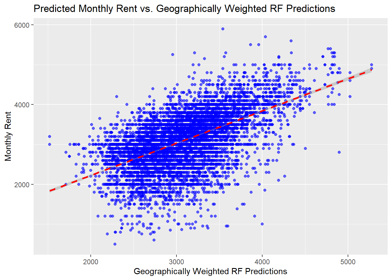

  theme_minimal() + 
  theme(plot.title = element_text(hjust = 0.5),  # Center the title
        axis.title = element_text(size = 12),  # Increase axis title size
        axis.text = element_text(size = 10))   # Increase axis text size

List of 136
 $ line                            :List of 6
  ..$ colour       : chr "black"
  ..$ linewidth    : num 0.5
  ..$ linetype     : num 1
  ..$ lineend      : chr "butt"
  ..$ arrow        : logi FALSE
  ..$ inherit.blank: logi TRUE
  ..- attr(*, "class")= chr [1:2] "element_line" "element"
 $ rect                            :List of 5
  ..$ fill         : chr "white"
  ..$ colour       : chr "black"
  ..$ linewidth    : num 0.5
  ..$ linetype     : num 1
  ..$ inherit.blank: logi TRUE
  ..- attr(*, "class")= chr [1:2] "element_rect" "element"
 $ text                            :List of 11
  ..$ family       : chr ""
  ..$ face         : chr "plain"
  ..$ colour       : chr "black"
  ..$ size         : num 11
  ..$ hjust        : num 0.5
  ..$ vjust        : num 0.5
  ..$ angle        : num 0
  ..$ lineheight   : num 0.9
  ..$ margin       : 'margin' num [1:4] 0points 0points 0points 0points
  .. ..- attr(*, "unit")= int 8
  ..$ debug        : logi FALSE
  ..$ inherit.blank: logi TRUE
  ..- attr(*, "class")= chr [1:2] "element_text" "element"
 $ title                           : NULL
 $ aspect.ratio                    : NULL
 $ axis.title                      :List of 11
  ..$ family       : NULL
  ..$ face         : NULL
  ..$ colour       : NULL
  ..$ size         : num 12
  ..$ hjust        : NULL
  ..$ vjust        : NULL
  ..$ angle        : NULL
  ..$ lineheight   : NULL
  ..$ margin       : NULL
  ..$ debug        : NULL
  ..$ inherit.blank: logi FALSE
  ..- attr(*, "class")= chr [1:2] "element_text" "element"
 $ axis.title.x                    :List of 11
  ..$ family       : NULL
  ..$ face         : NULL
  ..$ colour       : NULL
  ..$ size         : NULL
  ..$ hjust        : NULL
  ..$ vjust        : num 1
  ..$ angle        : NULL
  ..$ lineheight   : NULL
  ..$ margin       : 'margin' num [1:4] 2.75points 0points 0points 0points
  .. ..- attr(*, "unit")= int 8
  ..$ debug        : NULL
  ..$ inherit.blank: logi TRUE
  ..- attr(*, "class")= chr [1:2] "element_text" "element"
 $ axis.title.x.top                :List of 11
  ..$ family       : NULL
  ..$ face         : NULL
  ..$ colour       : NULL
  ..$ size         : NULL
  ..$ hjust        : NULL
  ..$ vjust        : num 0
  ..$ angle        : NULL
  ..$ lineheight   : NULL
  ..$ margin       : 'margin' num [1:4] 0points 0points 2.75points 0points
  .. ..- attr(*, "unit")= int 8
  ..$ debug        : NULL
  ..$ inherit.blank: logi TRUE
  ..- attr(*, "class")= chr [1:2] "element_text" "element"
 $ axis.title.x.bottom             : NULL
 $ axis.title.y                    :List of 11
  ..$ family       : NULL
  ..$ face         : NULL
  ..$ colour       : NULL
  ..$ size         : NULL
  ..$ hjust        : NULL
  ..$ vjust        : num 1
  ..$ angle        : num 90
  ..$ lineheight   : NULL
  ..$ margin       : 'margin' num [1:4] 0points 2.75points 0points 0points
  .. ..- attr(*, "unit")= int 8
  ..$ debug        : NULL
  ..$ inherit.blank: logi TRUE
  ..- attr(*, "class")= chr [1:2] "element_text" "element"
 $ axis.title.y.left               : NULL
 $ axis.title.y.right              :List of 11
  ..$ family       : NULL
  ..$ face         : NULL
  ..$ colour       : NULL
  ..$ size         : NULL
  ..$ hjust        : NULL
  ..$ vjust        : num 1
  ..$ angle        : num -90
  ..$ lineheight   : NULL
  ..$ margin       : 'margin' num [1:4] 0points 0points 0points 2.75points
  .. ..- attr(*, "unit")= int 8
  ..$ debug        : NULL
  ..$ inherit.blank: logi TRUE
  ..- attr(*, "class")= chr [1:2] "element_text" "element"
 $ axis.text                       :List of 11
  ..$ family       : NULL
  ..$ face         : NULL
  ..$ colour       : chr "grey30"
  ..$ size         : num 10
  ..$ hjust        : NULL
  ..$ vjust        : NULL
  ..$ angle        : NULL
  ..$ lineheight   : NULL
  ..$ margin       : NULL
  ..$ debug        : NULL
  ..$ inherit.blank: logi FALSE
  ..- attr(*, "class")= chr [1:2] "element_text" "element"
 $ axis.text.x                     :List of 11
  ..$ family       : NULL
  ..$ face         : NULL
  ..$ colour       : NULL
  ..$ size         : NULL
  ..$ hjust        : NULL
  ..$ vjust        : num 1
  ..$ angle        : NULL
  ..$ lineheight   : NULL
  ..$ margin       : 'margin' num [1:4] 2.2points 0points 0points 0points
  .. ..- attr(*, "unit")= int 8
  ..$ debug        : NULL
  ..$ inherit.blank: logi TRUE
  ..- attr(*, "class")= chr [1:2] "element_text" "element"
 $ axis.text.x.top                 :List of 11
  ..$ family       : NULL
  ..$ face         : NULL
  ..$ colour       : NULL
  ..$ size         : NULL
  ..$ hjust        : NULL
  ..$ vjust        : num 0
  ..$ angle        : NULL
  ..$ lineheight   : NULL
  ..$ margin       : 'margin' num [1:4] 0points 0points 2.2points 0points
  .. ..- attr(*, "unit")= int 8
  ..$ debug        : NULL
  ..$ inherit.blank: logi TRUE
  ..- attr(*, "class")= chr [1:2] "element_text" "element"
 $ axis.text.x.bottom              : NULL
 $ axis.text.y                     :List of 11
  ..$ family       : NULL
  ..$ face         : NULL
  ..$ colour       : NULL
  ..$ size         : NULL
  ..$ hjust        : num 1
  ..$ vjust        : NULL
  ..$ angle        : NULL
  ..$ lineheight   : NULL
  ..$ margin       : 'margin' num [1:4] 0points 2.2points 0points 0points
  .. ..- attr(*, "unit")= int 8
  ..$ debug        : NULL
  ..$ inherit.blank: logi TRUE
  ..- attr(*, "class")= chr [1:2] "element_text" "element"
 $ axis.text.y.left                : NULL
 $ axis.text.y.right               :List of 11
  ..$ family       : NULL
  ..$ face         : NULL
  ..$ colour       : NULL
  ..$ size         : NULL
  ..$ hjust        : num 0
  ..$ vjust        : NULL
  ..$ angle        : NULL
  ..$ lineheight   : NULL
  ..$ margin       : 'margin' num [1:4] 0points 0points 0points 2.2points
  .. ..- attr(*, "unit")= int 8
  ..$ debug        : NULL
  ..$ inherit.blank: logi TRUE
  ..- attr(*, "class")= chr [1:2] "element_text" "element"
 $ axis.text.theta                 : NULL
 $ axis.text.r                     :List of 11
  ..$ family       : NULL
  ..$ face         : NULL
  ..$ colour       : NULL
  ..$ size         : NULL
  ..$ hjust        : num 0.5
  ..$ vjust        : NULL
  ..$ angle        : NULL
  ..$ lineheight   : NULL
  ..$ margin       : 'margin' num [1:4] 0points 2.2points 0points 2.2points
  .. ..- attr(*, "unit")= int 8
  ..$ debug        : NULL
  ..$ inherit.blank: logi TRUE
  ..- attr(*, "class")= chr [1:2] "element_text" "element"
 $ axis.ticks                      : list()
  ..- attr(*, "class")= chr [1:2] "element_blank" "element"
 $ axis.ticks.x                    : NULL
 $ axis.ticks.x.top                : NULL
 $ axis.ticks.x.bottom             : NULL
 $ axis.ticks.y                    : NULL
 $ axis.ticks.y.left               : NULL
 $ axis.ticks.y.right              : NULL
 $ axis.ticks.theta                : NULL
 $ axis.ticks.r                    : NULL
 $ axis.minor.ticks.x.top          : NULL
 $ axis.minor.ticks.x.bottom       : NULL
 $ axis.minor.ticks.y.left         : NULL
 $ axis.minor.ticks.y.right        : NULL
 $ axis.minor.ticks.theta          : NULL
 $ axis.minor.ticks.r              : NULL
 $ axis.ticks.length               : 'simpleUnit' num 2.75points
  ..- attr(*, "unit")= int 8
 $ axis.ticks.length.x             : NULL
 $ axis.ticks.length.x.top         : NULL
 $ axis.ticks.length.x.bottom      : NULL
 $ axis.ticks.length.y             : NULL
 $ axis.ticks.length.y.left        : NULL
 $ axis.ticks.length.y.right       : NULL
 $ axis.ticks.length.theta         : NULL
 $ axis.ticks.length.r             : NULL
 $ axis.minor.ticks.length         : 'rel' num 0.75
 $ axis.minor.ticks.length.x       : NULL
 $ axis.minor.ticks.length.x.top   : NULL
 $ axis.minor.ticks.length.x.bottom: NULL
 $ axis.minor.ticks.length.y       : NULL
 $ axis.minor.ticks.length.y.left  : NULL
 $ axis.minor.ticks.length.y.right : NULL
 $ axis.minor.ticks.length.theta   : NULL
 $ axis.minor.ticks.length.r       : NULL
 $ axis.line                       : list()
  ..- attr(*, "class")= chr [1:2] "element_blank" "element"
 $ axis.line.x                     : NULL
 $ axis.line.x.top                 : NULL
 $ axis.line.x.bottom              : NULL
 $ axis.line.y                     : NULL
 $ axis.line.y.left                : NULL
 $ axis.line.y.right               : NULL
 $ axis.line.theta                 : NULL
 $ axis.line.r                     : NULL
 $ legend.background               : list()
  ..- attr(*, "class")= chr [1:2] "element_blank" "element"
 $ legend.margin                   : 'margin' num [1:4] 5.5points 5.5points 5.5points 5.5points
  ..- attr(*, "unit")= int 8
 $ legend.spacing                  : 'simpleUnit' num 11points
  ..- attr(*, "unit")= int 8
 $ legend.spacing.x                : NULL
 $ legend.spacing.y                : NULL
 $ legend.key                      : list()
  ..- attr(*, "class")= chr [1:2] "element_blank" "element"
 $ legend.key.size                 : 'simpleUnit' num 1.2lines
  ..- attr(*, "unit")= int 3
 $ legend.key.height               : NULL
 $ legend.key.width                : NULL
 $ legend.key.spacing              : 'simpleUnit' num 5.5points
  ..- attr(*, "unit")= int 8
 $ legend.key.spacing.x            : NULL
 $ legend.key.spacing.y            : NULL
 $ legend.frame                    : NULL
 $ legend.ticks                    : NULL
 $ legend.ticks.length             : 'rel' num 0.2
 $ legend.axis.line                : NULL
 $ legend.text                     :List of 11
  ..$ family       : NULL
  ..$ face         : NULL
  ..$ colour       : NULL
  ..$ size         : 'rel' num 0.8
  ..$ hjust        : NULL
  ..$ vjust        : NULL
  ..$ angle        : NULL
  ..$ lineheight   : NULL
  ..$ margin       : NULL
  ..$ debug        : NULL
  ..$ inherit.blank: logi TRUE
  ..- attr(*, "class")= chr [1:2] "element_text" "element"
 $ legend.text.position            : NULL
 $ legend.title                    :List of 11
  ..$ family       : NULL
  ..$ face         : NULL
  ..$ colour       : NULL
  ..$ size         : NULL
  ..$ hjust        : num 0
  ..$ vjust        : NULL
  ..$ angle        : NULL
  ..$ lineheight   : NULL
  ..$ margin       : NULL
  ..$ debug        : NULL
  ..$ inherit.blank: logi TRUE
  ..- attr(*, "class")= chr [1:2] "element_text" "element"
 $ legend.title.position           : NULL
 $ legend.position                 : chr "right"
 $ legend.position.inside          : NULL
 $ legend.direction                : NULL
 $ legend.byrow                    : NULL
 $ legend.justification            : chr "center"
 $ legend.justification.top        : NULL
 $ legend.justification.bottom     : NULL
 $ legend.justification.left       : NULL
 $ legend.justification.right      : NULL
 $ legend.justification.inside     : NULL
 $ legend.location                 : NULL
 $ legend.box                      : NULL
 $ legend.box.just                 : NULL
 $ legend.box.margin               : 'margin' num [1:4] 0cm 0cm 0cm 0cm
  ..- attr(*, "unit")= int 1
 $ legend.box.background           : list()
  ..- attr(*, "class")= chr [1:2] "element_blank" "element"
 $ legend.box.spacing              : 'simpleUnit' num 11points
  ..- attr(*, "unit")= int 8
  [list output truncated]
 - attr(*, "class")= chr [1:2] "theme" "gg"
 - attr(*, "complete")= logi TRUE
 - attr(*, "validate")= logi TRUE

3.9.5.2 Random Forest (RF) Model with Tuned Hyperparameters

Show the code

duplicate_columns <- names(test_data_rpt)[duplicated(names(test_data_rpt))]
test_data_rpt <- test_data_rpt[, !duplicated(names(test_data_rpt))]

ggplot(data = test_data_rpt, aes(x = prediction, y = monthly_rent)) +
  geom_point(alpha = 0.6, color = "blue") +  # Adjust point transparency and color
  geom_smooth(method = "lm", se = TRUE, color = "red", linetype = "dashed") +  # Best fit line
  labs(title = "Predicted Monthly Rent vs. Geographically Weighted RF Predictions",
       x = "Geographically Weighted RF Predictions",
       y = "Monthly Rent")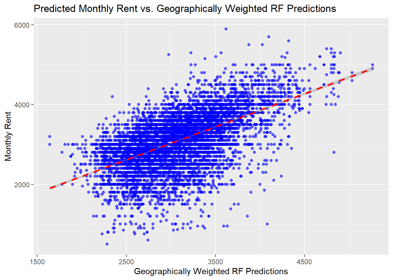

  theme_minimal() + 
  theme(plot.title = element_text(hjust = 0.5),  # Center the title
        axis.title = element_text(size = 12),  # Increase axis title size
        axis.text = element_text(size = 10))   # Increase axis text size

List of 136
 $ line                            :List of 6
  ..$ colour       : chr "black"
  ..$ linewidth    : num 0.5
  ..$ linetype     : num 1
  ..$ lineend      : chr "butt"
  ..$ arrow        : logi FALSE
  ..$ inherit.blank: logi TRUE
  ..- attr(*, "class")= chr [1:2] "element_line" "element"
 $ rect                            :List of 5
  ..$ fill         : chr "white"
  ..$ colour       : chr "black"
  ..$ linewidth    : num 0.5
  ..$ linetype     : num 1
  ..$ inherit.blank: logi TRUE
  ..- attr(*, "class")= chr [1:2] "element_rect" "element"
 $ text                            :List of 11
  ..$ family       : chr ""
  ..$ face         : chr "plain"
  ..$ colour       : chr "black"
  ..$ size         : num 11
  ..$ hjust        : num 0.5
  ..$ vjust        : num 0.5
  ..$ angle        : num 0
  ..$ lineheight   : num 0.9
  ..$ margin       : 'margin' num [1:4] 0points 0points 0points 0points
  .. ..- attr(*, "unit")= int 8
  ..$ debug        : logi FALSE
  ..$ inherit.blank: logi TRUE
  ..- attr(*, "class")= chr [1:2] "element_text" "element"
 $ title                           : NULL
 $ aspect.ratio                    : NULL
 $ axis.title                      :List of 11
  ..$ family       : NULL
  ..$ face         : NULL
  ..$ colour       : NULL
  ..$ size         : num 12
  ..$ hjust        : NULL
  ..$ vjust        : NULL
  ..$ angle        : NULL
  ..$ lineheight   : NULL
  ..$ margin       : NULL
  ..$ debug        : NULL
  ..$ inherit.blank: logi FALSE
  ..- attr(*, "class")= chr [1:2] "element_text" "element"
 $ axis.title.x                    :List of 11
  ..$ family       : NULL
  ..$ face         : NULL
  ..$ colour       : NULL
  ..$ size         : NULL
  ..$ hjust        : NULL
  ..$ vjust        : num 1
  ..$ angle        : NULL
  ..$ lineheight   : NULL
  ..$ margin       : 'margin' num [1:4] 2.75points 0points 0points 0points
  .. ..- attr(*, "unit")= int 8
  ..$ debug        : NULL
  ..$ inherit.blank: logi TRUE
  ..- attr(*, "class")= chr [1:2] "element_text" "element"
 $ axis.title.x.top                :List of 11
  ..$ family       : NULL
  ..$ face         : NULL
  ..$ colour       : NULL
  ..$ size         : NULL
  ..$ hjust        : NULL
  ..$ vjust        : num 0
  ..$ angle        : NULL
  ..$ lineheight   : NULL
  ..$ margin       : 'margin' num [1:4] 0points 0points 2.75points 0points
  .. ..- attr(*, "unit")= int 8
  ..$ debug        : NULL
  ..$ inherit.blank: logi TRUE
  ..- attr(*, "class")= chr [1:2] "element_text" "element"
 $ axis.title.x.bottom             : NULL
 $ axis.title.y                    :List of 11
  ..$ family       : NULL
  ..$ face         : NULL
  ..$ colour       : NULL
  ..$ size         : NULL
  ..$ hjust        : NULL
  ..$ vjust        : num 1
  ..$ angle        : num 90
  ..$ lineheight   : NULL
  ..$ margin       : 'margin' num [1:4] 0points 2.75points 0points 0points
  .. ..- attr(*, "unit")= int 8
  ..$ debug        : NULL
  ..$ inherit.blank: logi TRUE
  ..- attr(*, "class")= chr [1:2] "element_text" "element"
 $ axis.title.y.left               : NULL
 $ axis.title.y.right              :List of 11
  ..$ family       : NULL
  ..$ face         : NULL
  ..$ colour       : NULL
  ..$ size         : NULL
  ..$ hjust        : NULL
  ..$ vjust        : num 1
  ..$ angle        : num -90
  ..$ lineheight   : NULL
  ..$ margin       : 'margin' num [1:4] 0points 0points 0points 2.75points
  .. ..- attr(*, "unit")= int 8
  ..$ debug        : NULL
  ..$ inherit.blank: logi TRUE
  ..- attr(*, "class")= chr [1:2] "element_text" "element"
 $ axis.text                       :List of 11
  ..$ family       : NULL
  ..$ face         : NULL
  ..$ colour       : chr "grey30"
  ..$ size         : num 10
  ..$ hjust        : NULL
  ..$ vjust        : NULL
  ..$ angle        : NULL
  ..$ lineheight   : NULL
  ..$ margin       : NULL
  ..$ debug        : NULL
  ..$ inherit.blank: logi FALSE
  ..- attr(*, "class")= chr [1:2] "element_text" "element"
 $ axis.text.x                     :List of 11
  ..$ family       : NULL
  ..$ face         : NULL
  ..$ colour       : NULL
  ..$ size         : NULL
  ..$ hjust        : NULL
  ..$ vjust        : num 1
  ..$ angle        : NULL
  ..$ lineheight   : NULL
  ..$ margin       : 'margin' num [1:4] 2.2points 0points 0points 0points
  .. ..- attr(*, "unit")= int 8
  ..$ debug        : NULL
  ..$ inherit.blank: logi TRUE
  ..- attr(*, "class")= chr [1:2] "element_text" "element"
 $ axis.text.x.top                 :List of 11
  ..$ family       : NULL
  ..$ face         : NULL
  ..$ colour       : NULL
  ..$ size         : NULL
  ..$ hjust        : NULL
  ..$ vjust        : num 0
  ..$ angle        : NULL
  ..$ lineheight   : NULL
  ..$ margin       : 'margin' num [1:4] 0points 0points 2.2points 0points
  .. ..- attr(*, "unit")= int 8
  ..$ debug        : NULL
  ..$ inherit.blank: logi TRUE
  ..- attr(*, "class")= chr [1:2] "element_text" "element"
 $ axis.text.x.bottom              : NULL
 $ axis.text.y                     :List of 11
  ..$ family       : NULL
  ..$ face         : NULL
  ..$ colour       : NULL
  ..$ size         : NULL
  ..$ hjust        : num 1
  ..$ vjust        : NULL
  ..$ angle        : NULL
  ..$ lineheight   : NULL
  ..$ margin       : 'margin' num [1:4] 0points 2.2points 0points 0points
  .. ..- attr(*, "unit")= int 8
  ..$ debug        : NULL
  ..$ inherit.blank: logi TRUE
  ..- attr(*, "class")= chr [1:2] "element_text" "element"
 $ axis.text.y.left                : NULL
 $ axis.text.y.right               :List of 11
  ..$ family       : NULL
  ..$ face         : NULL
  ..$ colour       : NULL
  ..$ size         : NULL
  ..$ hjust        : num 0
  ..$ vjust        : NULL
  ..$ angle        : NULL
  ..$ lineheight   : NULL
  ..$ margin       : 'margin' num [1:4] 0points 0points 0points 2.2points
  .. ..- attr(*, "unit")= int 8
  ..$ debug        : NULL
  ..$ inherit.blank: logi TRUE
  ..- attr(*, "class")= chr [1:2] "element_text" "element"
 $ axis.text.theta                 : NULL
 $ axis.text.r                     :List of 11
  ..$ family       : NULL
  ..$ face         : NULL
  ..$ colour       : NULL
  ..$ size         : NULL
  ..$ hjust        : num 0.5
  ..$ vjust        : NULL
  ..$ angle        : NULL
  ..$ lineheight   : NULL
  ..$ margin       : 'margin' num [1:4] 0points 2.2points 0points 2.2points
  .. ..- attr(*, "unit")= int 8
  ..$ debug        : NULL
  ..$ inherit.blank: logi TRUE
  ..- attr(*, "class")= chr [1:2] "element_text" "element"
 $ axis.ticks                      : list()
  ..- attr(*, "class")= chr [1:2] "element_blank" "element"
 $ axis.ticks.x                    : NULL
 $ axis.ticks.x.top                : NULL
 $ axis.ticks.x.bottom             : NULL
 $ axis.ticks.y                    : NULL
 $ axis.ticks.y.left               : NULL
 $ axis.ticks.y.right              : NULL
 $ axis.ticks.theta                : NULL
 $ axis.ticks.r                    : NULL
 $ axis.minor.ticks.x.top          : NULL
 $ axis.minor.ticks.x.bottom       : NULL
 $ axis.minor.ticks.y.left         : NULL
 $ axis.minor.ticks.y.right        : NULL
 $ axis.minor.ticks.theta          : NULL
 $ axis.minor.ticks.r              : NULL
 $ axis.ticks.length               : 'simpleUnit' num 2.75points
  ..- attr(*, "unit")= int 8
 $ axis.ticks.length.x             : NULL
 $ axis.ticks.length.x.top         : NULL
 $ axis.ticks.length.x.bottom      : NULL
 $ axis.ticks.length.y             : NULL
 $ axis.ticks.length.y.left        : NULL
 $ axis.ticks.length.y.right       : NULL
 $ axis.ticks.length.theta         : NULL
 $ axis.ticks.length.r             : NULL
 $ axis.minor.ticks.length         : 'rel' num 0.75
 $ axis.minor.ticks.length.x       : NULL
 $ axis.minor.ticks.length.x.top   : NULL
 $ axis.minor.ticks.length.x.bottom: NULL
 $ axis.minor.ticks.length.y       : NULL
 $ axis.minor.ticks.length.y.left  : NULL
 $ axis.minor.ticks.length.y.right : NULL
 $ axis.minor.ticks.length.theta   : NULL
 $ axis.minor.ticks.length.r       : NULL
 $ axis.line                       : list()
  ..- attr(*, "class")= chr [1:2] "element_blank" "element"
 $ axis.line.x                     : NULL
 $ axis.line.x.top                 : NULL
 $ axis.line.x.bottom              : NULL
 $ axis.line.y                     : NULL
 $ axis.line.y.left                : NULL
 $ axis.line.y.right               : NULL
 $ axis.line.theta                 : NULL
 $ axis.line.r                     : NULL
 $ legend.background               : list()
  ..- attr(*, "class")= chr [1:2] "element_blank" "element"
 $ legend.margin                   : 'margin' num [1:4] 5.5points 5.5points 5.5points 5.5points
  ..- attr(*, "unit")= int 8
 $ legend.spacing                  : 'simpleUnit' num 11points
  ..- attr(*, "unit")= int 8
 $ legend.spacing.x                : NULL
 $ legend.spacing.y                : NULL
 $ legend.key                      : list()
  ..- attr(*, "class")= chr [1:2] "element_blank" "element"
 $ legend.key.size                 : 'simpleUnit' num 1.2lines
  ..- attr(*, "unit")= int 3
 $ legend.key.height               : NULL
 $ legend.key.width                : NULL
 $ legend.key.spacing              : 'simpleUnit' num 5.5points
  ..- attr(*, "unit")= int 8
 $ legend.key.spacing.x            : NULL
 $ legend.key.spacing.y            : NULL
 $ legend.frame                    : NULL
 $ legend.ticks                    : NULL
 $ legend.ticks.length             : 'rel' num 0.2
 $ legend.axis.line                : NULL
 $ legend.text                     :List of 11
  ..$ family       : NULL
  ..$ face         : NULL
  ..$ colour       : NULL
  ..$ size         : 'rel' num 0.8
  ..$ hjust        : NULL
  ..$ vjust        : NULL
  ..$ angle        : NULL
  ..$ lineheight   : NULL
  ..$ margin       : NULL
  ..$ debug        : NULL
  ..$ inherit.blank: logi TRUE
  ..- attr(*, "class")= chr [1:2] "element_text" "element"
 $ legend.text.position            : NULL
 $ legend.title                    :List of 11
  ..$ family       : NULL
  ..$ face         : NULL
  ..$ colour       : NULL
  ..$ size         : NULL
  ..$ hjust        : num 0
  ..$ vjust        : NULL
  ..$ angle        : NULL
  ..$ lineheight   : NULL
  ..$ margin       : NULL
  ..$ debug        : NULL
  ..$ inherit.blank: logi TRUE
  ..- attr(*, "class")= chr [1:2] "element_text" "element"
 $ legend.title.position           : NULL
 $ legend.position                 : chr "right"
 $ legend.position.inside          : NULL
 $ legend.direction                : NULL
 $ legend.byrow                    : NULL
 $ legend.justification            : chr "center"
 $ legend.justification.top        : NULL
 $ legend.justification.bottom     : NULL
 $ legend.justification.left       : NULL
 $ legend.justification.right      : NULL
 $ legend.justification.inside     : NULL
 $ legend.location                 : NULL
 $ legend.box                      : NULL
 $ legend.box.just                 : NULL
 $ legend.box.margin               : 'margin' num [1:4] 0cm 0cm 0cm 0cm
  ..- attr(*, "unit")= int 1
 $ legend.box.background           : list()
  ..- attr(*, "class")= chr [1:2] "element_blank" "element"
 $ legend.box.spacing              : 'simpleUnit' num 11points
  ..- attr(*, "unit")= int 8
  [list output truncated]
 - attr(*, "class")= chr [1:2] "theme" "gg"
 - attr(*, "complete")= logi TRUE
 - attr(*, "validate")= logi TRUE

3.9.5.3 Geographical Random Forest (GRF) Model

Show the code

duplicate_columns <- names(test_data_gp)[duplicated(names(test_data_gp))]
test_data_gp <- test_data_gp[, !duplicated(names(test_data_gp))]

ggplot(data = test_data_gp, aes(x = gwRF_pred, y = monthly_rent)) +
  geom_point(alpha = 0.6, color = "blue") +  # Adjust point transparency and color
  geom_smooth(method = "lm", se = TRUE, color = "red", linetype = "dashed") +  # Best fit line
  labs(title = "Predicted Monthly Rent vs. Geographically Weighted RF Predictions",
       x = "Geographically Weighted RF Predictions",
       y = "Monthly Rent")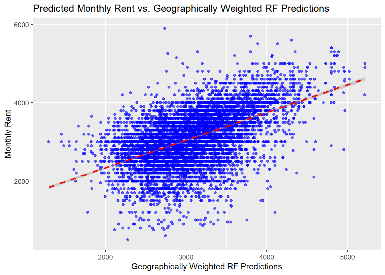

  theme_minimal() + 
  theme(plot.title = element_text(hjust = 0.5),  # Center the title
        axis.title = element_text(size = 12),  # Increase axis title size
        axis.text = element_text(size = 10))   # Increase axis text size

List of 136
 $ line                            :List of 6
  ..$ colour       : chr "black"
  ..$ linewidth    : num 0.5
  ..$ linetype     : num 1
  ..$ lineend      : chr "butt"
  ..$ arrow        : logi FALSE
  ..$ inherit.blank: logi TRUE
  ..- attr(*, "class")= chr [1:2] "element_line" "element"
 $ rect                            :List of 5
  ..$ fill         : chr "white"
  ..$ colour       : chr "black"
  ..$ linewidth    : num 0.5
  ..$ linetype     : num 1
  ..$ inherit.blank: logi TRUE
  ..- attr(*, "class")= chr [1:2] "element_rect" "element"
 $ text                            :List of 11
  ..$ family       : chr ""
  ..$ face         : chr "plain"
  ..$ colour       : chr "black"
  ..$ size         : num 11
  ..$ hjust        : num 0.5
  ..$ vjust        : num 0.5
  ..$ angle        : num 0
  ..$ lineheight   : num 0.9
  ..$ margin       : 'margin' num [1:4] 0points 0points 0points 0points
  .. ..- attr(*, "unit")= int 8
  ..$ debug        : logi FALSE
  ..$ inherit.blank: logi TRUE
  ..- attr(*, "class")= chr [1:2] "element_text" "element"
 $ title                           : NULL
 $ aspect.ratio                    : NULL
 $ axis.title                      :List of 11
  ..$ family       : NULL
  ..$ face         : NULL
  ..$ colour       : NULL
  ..$ size         : num 12
  ..$ hjust        : NULL
  ..$ vjust        : NULL
  ..$ angle        : NULL
  ..$ lineheight   : NULL
  ..$ margin       : NULL
  ..$ debug        : NULL
  ..$ inherit.blank: logi FALSE
  ..- attr(*, "class")= chr [1:2] "element_text" "element"
 $ axis.title.x                    :List of 11
  ..$ family       : NULL
  ..$ face         : NULL
  ..$ colour       : NULL
  ..$ size         : NULL
  ..$ hjust        : NULL
  ..$ vjust        : num 1
  ..$ angle        : NULL
  ..$ lineheight   : NULL
  ..$ margin       : 'margin' num [1:4] 2.75points 0points 0points 0points
  .. ..- attr(*, "unit")= int 8
  ..$ debug        : NULL
  ..$ inherit.blank: logi TRUE
  ..- attr(*, "class")= chr [1:2] "element_text" "element"
 $ axis.title.x.top                :List of 11
  ..$ family       : NULL
  ..$ face         : NULL
  ..$ colour       : NULL
  ..$ size         : NULL
  ..$ hjust        : NULL
  ..$ vjust        : num 0
  ..$ angle        : NULL
  ..$ lineheight   : NULL
  ..$ margin       : 'margin' num [1:4] 0points 0points 2.75points 0points
  .. ..- attr(*, "unit")= int 8
  ..$ debug        : NULL
  ..$ inherit.blank: logi TRUE
  ..- attr(*, "class")= chr [1:2] "element_text" "element"
 $ axis.title.x.bottom             : NULL
 $ axis.title.y                    :List of 11
  ..$ family       : NULL
  ..$ face         : NULL
  ..$ colour       : NULL
  ..$ size         : NULL
  ..$ hjust        : NULL
  ..$ vjust        : num 1
  ..$ angle        : num 90
  ..$ lineheight   : NULL
  ..$ margin       : 'margin' num [1:4] 0points 2.75points 0points 0points
  .. ..- attr(*, "unit")= int 8
  ..$ debug        : NULL
  ..$ inherit.blank: logi TRUE
  ..- attr(*, "class")= chr [1:2] "element_text" "element"
 $ axis.title.y.left               : NULL
 $ axis.title.y.right              :List of 11
  ..$ family       : NULL
  ..$ face         : NULL
  ..$ colour       : NULL
  ..$ size         : NULL
  ..$ hjust        : NULL
  ..$ vjust        : num 1
  ..$ angle        : num -90
  ..$ lineheight   : NULL
  ..$ margin       : 'margin' num [1:4] 0points 0points 0points 2.75points
  .. ..- attr(*, "unit")= int 8
  ..$ debug        : NULL
  ..$ inherit.blank: logi TRUE
  ..- attr(*, "class")= chr [1:2] "element_text" "element"
 $ axis.text                       :List of 11
  ..$ family       : NULL
  ..$ face         : NULL
  ..$ colour       : chr "grey30"
  ..$ size         : num 10
  ..$ hjust        : NULL
  ..$ vjust        : NULL
  ..$ angle        : NULL
  ..$ lineheight   : NULL
  ..$ margin       : NULL
  ..$ debug        : NULL
  ..$ inherit.blank: logi FALSE
  ..- attr(*, "class")= chr [1:2] "element_text" "element"
 $ axis.text.x                     :List of 11
  ..$ family       : NULL
  ..$ face         : NULL
  ..$ colour       : NULL
  ..$ size         : NULL
  ..$ hjust        : NULL
  ..$ vjust        : num 1
  ..$ angle        : NULL
  ..$ lineheight   : NULL
  ..$ margin       : 'margin' num [1:4] 2.2points 0points 0points 0points
  .. ..- attr(*, "unit")= int 8
  ..$ debug        : NULL
  ..$ inherit.blank: logi TRUE
  ..- attr(*, "class")= chr [1:2] "element_text" "element"
 $ axis.text.x.top                 :List of 11
  ..$ family       : NULL
  ..$ face         : NULL
  ..$ colour       : NULL
  ..$ size         : NULL
  ..$ hjust        : NULL
  ..$ vjust        : num 0
  ..$ angle        : NULL
  ..$ lineheight   : NULL
  ..$ margin       : 'margin' num [1:4] 0points 0points 2.2points 0points
  .. ..- attr(*, "unit")= int 8
  ..$ debug        : NULL
  ..$ inherit.blank: logi TRUE
  ..- attr(*, "class")= chr [1:2] "element_text" "element"
 $ axis.text.x.bottom              : NULL
 $ axis.text.y                     :List of 11
  ..$ family       : NULL
  ..$ face         : NULL
  ..$ colour       : NULL
  ..$ size         : NULL
  ..$ hjust        : num 1
  ..$ vjust        : NULL
  ..$ angle        : NULL
  ..$ lineheight   : NULL
  ..$ margin       : 'margin' num [1:4] 0points 2.2points 0points 0points
  .. ..- attr(*, "unit")= int 8
  ..$ debug        : NULL
  ..$ inherit.blank: logi TRUE
  ..- attr(*, "class")= chr [1:2] "element_text" "element"
 $ axis.text.y.left                : NULL
 $ axis.text.y.right               :List of 11
  ..$ family       : NULL
  ..$ face         : NULL
  ..$ colour       : NULL
  ..$ size         : NULL
  ..$ hjust        : num 0
  ..$ vjust        : NULL
  ..$ angle        : NULL
  ..$ lineheight   : NULL
  ..$ margin       : 'margin' num [1:4] 0points 0points 0points 2.2points
  .. ..- attr(*, "unit")= int 8
  ..$ debug        : NULL
  ..$ inherit.blank: logi TRUE
  ..- attr(*, "class")= chr [1:2] "element_text" "element"
 $ axis.text.theta                 : NULL
 $ axis.text.r                     :List of 11
  ..$ family       : NULL
  ..$ face         : NULL
  ..$ colour       : NULL
  ..$ size         : NULL
  ..$ hjust        : num 0.5
  ..$ vjust        : NULL
  ..$ angle        : NULL
  ..$ lineheight   : NULL
  ..$ margin       : 'margin' num [1:4] 0points 2.2points 0points 2.2points
  .. ..- attr(*, "unit")= int 8
  ..$ debug        : NULL
  ..$ inherit.blank: logi TRUE
  ..- attr(*, "class")= chr [1:2] "element_text" "element"
 $ axis.ticks                      : list()
  ..- attr(*, "class")= chr [1:2] "element_blank" "element"
 $ axis.ticks.x                    : NULL
 $ axis.ticks.x.top                : NULL
 $ axis.ticks.x.bottom             : NULL
 $ axis.ticks.y                    : NULL
 $ axis.ticks.y.left               : NULL
 $ axis.ticks.y.right              : NULL
 $ axis.ticks.theta                : NULL
 $ axis.ticks.r                    : NULL
 $ axis.minor.ticks.x.top          : NULL
 $ axis.minor.ticks.x.bottom       : NULL
 $ axis.minor.ticks.y.left         : NULL
 $ axis.minor.ticks.y.right        : NULL
 $ axis.minor.ticks.theta          : NULL
 $ axis.minor.ticks.r              : NULL
 $ axis.ticks.length               : 'simpleUnit' num 2.75points
  ..- attr(*, "unit")= int 8
 $ axis.ticks.length.x             : NULL
 $ axis.ticks.length.x.top         : NULL
 $ axis.ticks.length.x.bottom      : NULL
 $ axis.ticks.length.y             : NULL
 $ axis.ticks.length.y.left        : NULL
 $ axis.ticks.length.y.right       : NULL
 $ axis.ticks.length.theta         : NULL
 $ axis.ticks.length.r             : NULL
 $ axis.minor.ticks.length         : 'rel' num 0.75
 $ axis.minor.ticks.length.x       : NULL
 $ axis.minor.ticks.length.x.top   : NULL
 $ axis.minor.ticks.length.x.bottom: NULL
 $ axis.minor.ticks.length.y       : NULL
 $ axis.minor.ticks.length.y.left  : NULL
 $ axis.minor.ticks.length.y.right : NULL
 $ axis.minor.ticks.length.theta   : NULL
 $ axis.minor.ticks.length.r       : NULL
 $ axis.line                       : list()
  ..- attr(*, "class")= chr [1:2] "element_blank" "element"
 $ axis.line.x                     : NULL
 $ axis.line.x.top                 : NULL
 $ axis.line.x.bottom              : NULL
 $ axis.line.y                     : NULL
 $ axis.line.y.left                : NULL
 $ axis.line.y.right               : NULL
 $ axis.line.theta                 : NULL
 $ axis.line.r                     : NULL
 $ legend.background               : list()
  ..- attr(*, "class")= chr [1:2] "element_blank" "element"
 $ legend.margin                   : 'margin' num [1:4] 5.5points 5.5points 5.5points 5.5points
  ..- attr(*, "unit")= int 8
 $ legend.spacing                  : 'simpleUnit' num 11points
  ..- attr(*, "unit")= int 8
 $ legend.spacing.x                : NULL
 $ legend.spacing.y                : NULL
 $ legend.key                      : list()
  ..- attr(*, "class")= chr [1:2] "element_blank" "element"
 $ legend.key.size                 : 'simpleUnit' num 1.2lines
  ..- attr(*, "unit")= int 3
 $ legend.key.height               : NULL
 $ legend.key.width                : NULL
 $ legend.key.spacing              : 'simpleUnit' num 5.5points
  ..- attr(*, "unit")= int 8
 $ legend.key.spacing.x            : NULL
 $ legend.key.spacing.y            : NULL
 $ legend.frame                    : NULL
 $ legend.ticks                    : NULL
 $ legend.ticks.length             : 'rel' num 0.2
 $ legend.axis.line                : NULL
 $ legend.text                     :List of 11
  ..$ family       : NULL
  ..$ face         : NULL
  ..$ colour       : NULL
  ..$ size         : 'rel' num 0.8
  ..$ hjust        : NULL
  ..$ vjust        : NULL
  ..$ angle        : NULL
  ..$ lineheight   : NULL
  ..$ margin       : NULL
  ..$ debug        : NULL
  ..$ inherit.blank: logi TRUE
  ..- attr(*, "class")= chr [1:2] "element_text" "element"
 $ legend.text.position            : NULL
 $ legend.title                    :List of 11
  ..$ family       : NULL
  ..$ face         : NULL
  ..$ colour       : NULL
  ..$ size         : NULL
  ..$ hjust        : num 0
  ..$ vjust        : NULL
  ..$ angle        : NULL
  ..$ lineheight   : NULL
  ..$ margin       : NULL
  ..$ debug        : NULL
  ..$ inherit.blank: logi TRUE
  ..- attr(*, "class")= chr [1:2] "element_text" "element"
 $ legend.title.position           : NULL
 $ legend.position                 : chr "right"
 $ legend.position.inside          : NULL
 $ legend.direction                : NULL
 $ legend.byrow                    : NULL
 $ legend.justification            : chr "center"
 $ legend.justification.top        : NULL
 $ legend.justification.bottom     : NULL
 $ legend.justification.left       : NULL
 $ legend.justification.right      : NULL
 $ legend.justification.inside     : NULL
 $ legend.location                 : NULL
 $ legend.box                      : NULL
 $ legend.box.just                 : NULL
 $ legend.box.margin               : 'margin' num [1:4] 0cm 0cm 0cm 0cm
  ..- attr(*, "unit")= int 1
 $ legend.box.background           : list()
  ..- attr(*, "class")= chr [1:2] "element_blank" "element"
 $ legend.box.spacing              : 'simpleUnit' num 11points
  ..- attr(*, "unit")= int 8
  [list output truncated]
 - attr(*, "class")= chr [1:2] "theme" "gg"
 - attr(*, "complete")= logi TRUE
 - attr(*, "validate")= logi TRUE

Notes

With the different predictive models, users can choose the model that best fits their specific needs, depending on their requirements for accuracy, interpretability, or spatial relevance. Each model provides distinct benefits:

Standard Random Forest (RF): Offers a straightforward approach, balancing interpretability and predictive power with little calibration. It’s useful for users looking for a quick and reliable model without the need for significant adjustments.
Tuned Random Forest (RF with Tuned Hyperparameters): By focusing on the most impactful predictors and fine-tuning parameters like mtry and min.node.size, this model aims to achieve higher prediction accuracy. This is ideal for users who want an optimized model for maximum performance.
Geographic Random Forest (GRF): The geographically weighted RF model accounts for spatial differences in predictor effects, making it ideal for predictions where location plays a critical role, such as real estate or environmental modeling. Users interested in localized predictions would find this model particularly beneficial.

3.9.6 Summary and Practical Application

Each calibrated model provides a different lens through which HDB rental prices can be understood and predicted. For practical application:

For general insights, the Standard RF model may suffice.
For users seeking finer accuracy in specific feature relationships, the Tuned RF model provides a refined approach.
For users interested in spatial variation, the GRF model offers insights into how geographical context influences rent, making it highly applicable to real estate forecasting.

3.9.7 UI Design

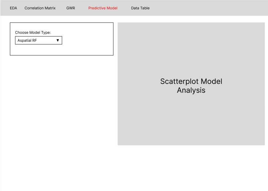
3.9.7.1 Scatterplot Model Analysis

Users would be able to explore the scatterplot model analysis of the various models. This setup allows users to visualise the comparison of RF models directly within the main panel and reference selection guidance. Only one plot is shown at a time, based on their selection, so as to not overwhelm them.

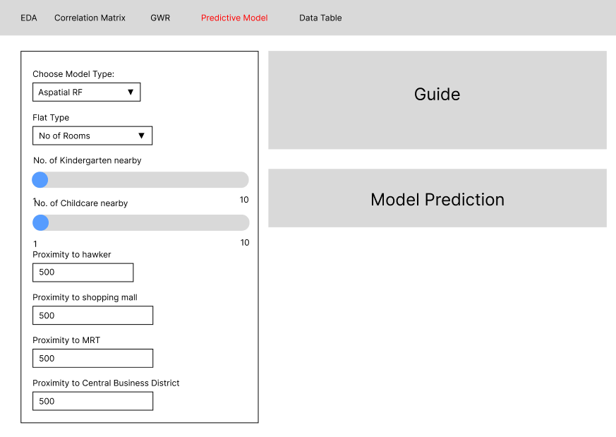
3.9.7.2 Predictive Models

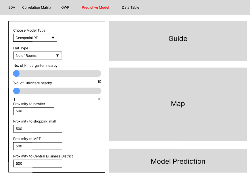
The guide section provides users with step-by-step instructions on how to navigate the UI, making the interface more intuitive.

The side panel (and the Map section for Geospatial model types) would simulate the functions of a calculator, where users would be able to input certain aspects of the their ideal HDB rental location to determine a likely monthly rental cost. Together this would provide users with a clearer understanding of how to interact with the tool and a polished output section for viewing predictions

This approach aims to provide a dynamic and intuitive way to input model parameters and view rental price predictions for different HDB flats in Singapore.

Take-home Exercise 3: Geographically Weighted Predictive Models: Rental price prediction based on location based data

3.1 Overview

3.2 Getting Started

3.3 Importing Data into R

3.4 Computing Correlation Matrix

3.5 Building a non-spatial multiple linear regression

3.6 Constructing the adaptive bandwidth gwr model

1. Global Regression Results

2. GWR Results

3. Diagnostics

3.7 Preparing coordinates data

3.7.1 Extracting coordinates data

3.7.2 Data Preparation

3.8 Calibrating Models

3.8.1 Calibrating using training data

3.8.2 Calibrating Random Forest (RF) Model

3.8.3 Calibrating Random Forest (RF) Model with Tuned Hyperparameters

3.8.4 Calibrating Geographical Random Forest (GRF) Model

3.9 Predicting by using test data

3.9.1 Preparing the test data

3.9.2 Predicting with test data

3.9.3 Formatting Prediction Outputs

3.9.4 Evaluating Model Accuracy with RMSE and MAE

3.9.4.1 Accuracy of Random Forest (RF) Model

3.9.4.2 Accuracy of Random Forest (RF) Model with Tuned Hyperparameters

3.9.4.3 Accuracy of Geographical Random Forest (GRF) Model

3.9.5 Visualising the predicted values

3.9.5.1 Random Forest (RF) Model

3.9.5.2 Random Forest (RF) Model with Tuned Hyperparameters

3.9.5.3 Geographical Random Forest (GRF) Model

3.9.6 Summary and Practical Application

3.9.7 UI Design

3.9.7.1 Scatterplot Model Analysis

3.9.7.2 Predictive Models

Aspatial Model Type

Geospatial Model Type