pacman::p_load(sf, raster, spatstat, sparr, tmap, tidyverse)In Class exercise 4
Analysis
R
sf
tidyverse
4.0 Overview
A spatio-temporal point process (also called space-time or spatial-temporal point process) is a random collection of points, where each point represents the time and location of an event. Examples of events include incidence of disease, sightings or births of a species, or the occurrences of fires, earthquakes, lightning strikes, tsunamis, or volcanic eruptions.
The analysis of spatio-temporal point patterns is becoming increasingly necessary, given the rapid emergence of geographically and temporally indexed data in a wide range of fields. Several spatio-temporal point patterns analysis methods have been introduced and implemented in R in the last ten years. This chapter shows how various R packages can be combined to run a set of spatio-temporal point pattern analyses in a guided and intuitive way. A real world forest fire events in Kepulauan Bangka Belitung, Indonesia from 1st January 2023 to 31st December 2023 is used to illustrate the methods, procedures and interpretations.
4.1 Learning Outcome
4.1.1 The research questions
The specific question we would like to answer is:
are the locations of forest fire in Kepulauan Bangka Belitung spatial and spatio-temporally independent?
if the answer is NO, where and when the observed forest fire locations tend to cluster?
4.1.2 The data
For the purpose of this exercise, two data sets are used, they are:
forestfires, a csv file provides locations of forest fire detected from the Moderate Resolution Imaging Spectroradiometer (MODIS) sensor data. The data are downloaded from Fire Information for Resource Management System. For the purpose of this exercise, only forest fires within Kepulauan Bangka Belitung will be used.
Kepulauan_Bangka_Belitung, an ESRI shapefile showing the sub-district (i.e. kelurahan) boundary of Kepulauan Bangka Belitung. The data set was downloaded from Indonesia Geospatial portal. The original data covers the whole Indonesia. For the purpose of this exercise, only sub-districts within Kepulauan Bangka Belitung are extracted.
4.2 Installing and Loading the R packages
For the purpose of this study, five R packages will be used. They are:
rgdal for importing geospatial data in GIS file format such as shapefile into R and save them as Spatial*DataFrame,
maptools for converting Spatial* object into ppp object,
raster for handling raster data in R,
sparr provides functions to estimate fixed and adaptive kernel-smooth spatial relative risk surfaces via the density-ratio method and perform subsequent inferences,
spatstat for performing Spatial Point Patterns Analysis such as kcross, Lcross, etc., and
tmap for producing cartographic quality thematic maps.
4.3 Importing data into R
4.3.1 Importing and Preparing Forest Fire shapeful
kbb_sf <- st_read(dsn = "data/In-class_Ex04",
                  layer = "Kepulauan_Bangka_Belitung") %>%
  st_union() %>%
  st_zm(drop = TRUE, what = "ZM") %>% # dropping the Z-value
  st_transform(crs = 32748)
Reading layer `Kepulauan_Bangka_Belitung' from data source
`C:\Users\blzll\OneDrive\Desktop\Y3S1\IS415\Quarto\IS415\In-class_Ex\data\In-class_Ex04'
using driver `ESRI Shapefile'
Simple feature collection with 298 features and 27 fields
Geometry type: POLYGON
Dimension: XYZ
Bounding box: xmin: 105.1085 ymin: -3.116593 xmax: 106.8488 ymax: -1.501603
z_range: zmin: 0 zmax: 0
Geodetic CRS: WGS 84summary(kbb_sf) MULTIPOLYGON epsg:32748 +proj=utm ...
1 0 0 Furthermore we create an owin object from the sf data type
kbb_owin <- as.owin(kbb_sf)
kbb_owin
window: polygonal boundary
enclosing rectangle: [512066.8, 705559.4] x [9655398, 9834006] unitsTo ensure that the output is an owin object
class(kbb_owin)[1] "owin"4.3.2 Importing and Preparing Forest Fire data
Next we will import the forest data set into R:
fire_sf <- read_csv("data/In-class_Ex04/forestfires.csv") %>%
  st_as_sf(coords = c("longitude", "latitude"),
           crs = 4326) %>%
  st_transform(crs = 32748)
Because ppp object only accept numerical or character as mark. The code below is used to transform acq_date data type to numeric.
fire_sf <- fire_sf %>%
  mutate("DayofYear" = yday(acq_date)) %>%
  mutate("Month_num" = month(acq_date)) %>%
  mutate("Month_fac" = month(acq_date, label = TRUE, abbr = FALSE))

summary(fire_sf)
brightness scan track acq_date
Min. :300.3 Min. :1.000 Min. :1.000 Min. :2023-01-10
1st Qu.:314.3 1st Qu.:1.000 1st Qu.:1.000 1st Qu.:2023-08-01
Median :318.7 Median :1.100 Median :1.100 Median :2023-09-15
Mean :320.9 Mean :1.315 Mean :1.119 Mean :2023-09-02
3rd Qu.:324.7 3rd Qu.:1.400 3rd Qu.:1.200 3rd Qu.:2023-10-14
Max. :396.2 Max. :4.200 Max. :1.900 Max. :2023-12-18
acq_time satellite instrument confidence
Min. : 248 Length:741 Length:741 Min. : 0.0
1st Qu.: 633 Class :character Class :character 1st Qu.: 57.0
Median : 649 Mode :character Mode :character Median : 68.0
Mean : 731 Mean : 65.6
3rd Qu.: 659 3rd Qu.: 77.0
Max. :1915 Max. :100.0
version bright_t31 frp daynight type
Min. :61.03 Min. :274.9 Min. : 3.0 Length:741 Min. :0
1st Qu.:61.03 1st Qu.:293.6 1st Qu.: 8.4 Class :character 1st Qu.:0
Median :61.03 Median :296.6 Median : 13.2 Mode :character Median :0
Mean :61.03 Mean :296.1 Mean : 20.1 Mean :0
3rd Qu.:61.03 3rd Qu.:299.2 3rd Qu.: 21.8 3rd Qu.:0
Max. :61.03 Max. :311.2 Max. :220.2 Max. :0
geometry DayofYear Month_num Month_fac
POINT :741 Min. : 10.0 Min. : 1.000 October :185
epsg:32748 : 0 1st Qu.:213.0 1st Qu.: 8.000 September:146
+proj=utm ...: 0 Median :258.0 Median : 9.000 August :143
Mean :245.9 Mean : 8.579 November : 88
3rd Qu.:287.0 3rd Qu.:10.000 July : 79
Max. :352.0 Max. :12.000 June : 34
(Other) : 66 4.4 Visualising the Fire Points
tm_shape(kbb_sf)+
  tm_polygons() +
  tm_shape(fire_sf) +
  tm_dots()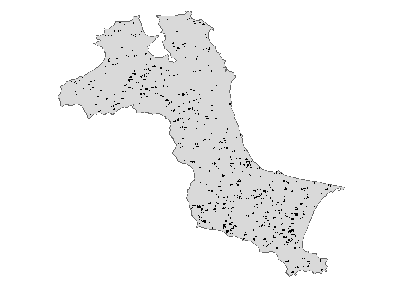
We will then prepare a point symbol map showing the monthly geographic distribution of forest fires in 2023. The map should look similar to the figure below.
tm_shape(kbb_sf)+
  tm_polygons()+
  tm_shape(fire_sf)+
  tm_dots(size = 0.1)+
  tm_facets(by="Month_fac", free.coords = FALSE, drop.units = FALSE)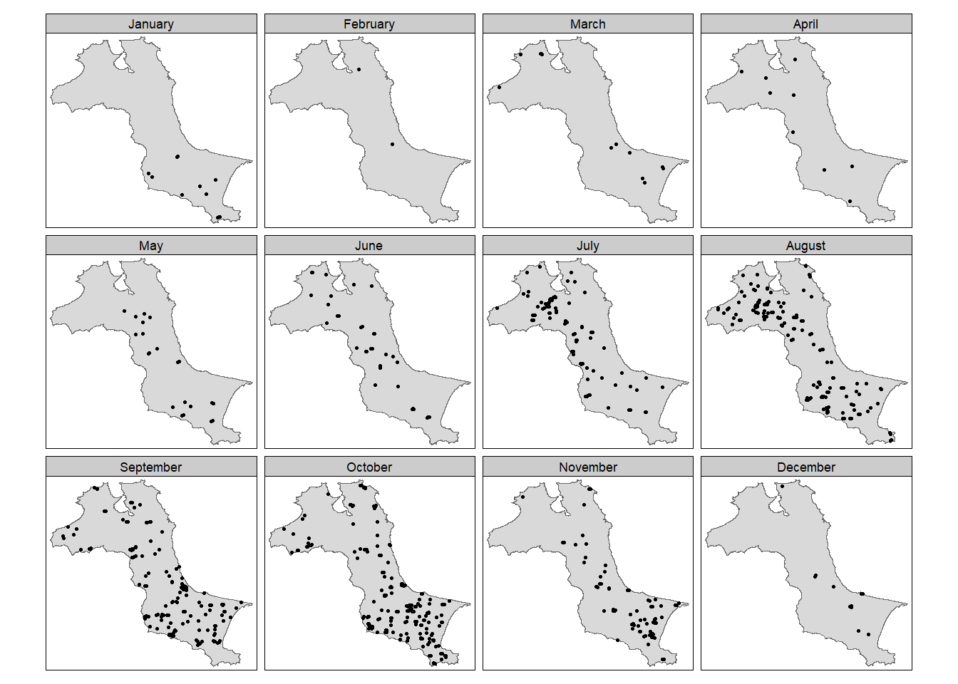
4.5 Extracting forest fire by month
The code chunk below is used to remove the unwanted fields from the fire_sf sf data frame. This is because as.ppp() only need the mark field and geometry field from the input sf data frame.
fire_month <- fire_sf %>%
  select(Month_num)
4.5.1 Creating ppp
The code chunk below is used to derive a ppp object called fire_month from fire_month sf data frame
fire_month_ppp <- as.ppp(fire_month)
fire_month_ppp
Marked planar point pattern: 741 points
marks are numeric, of storage type 'double'
window: rectangle = [521564.1, 695791] x [9658137, 9828767] units4.5.2 Creating Owin object
The code chunk below is used to combine origin_am_ppp and am_owin_objects into one.
fire_month_owin <- fire_month_ppp[kbb_owin]
summary(fire_month_owin)
Marked planar point pattern: 741 points
Average intensity 6.424519e-08 points per square unit
Coordinates are given to 10 decimal places
marks are numeric, of type 'double'
Summary:
Min. 1st Qu. Median Mean 3rd Qu. Max.
1.000 8.000 9.000 8.579 10.000 12.000
Window: polygonal boundary
2 separate polygons (no holes)
vertices area relative.area
polygon 1 47493 11533600000 1.00e+00
polygon 2 256 306427 2.66e-05
enclosing rectangle: [512066.8, 705559.4] x [9655398, 9834006] units
(193500 x 178600 units)
Window area = 11533900000 square units
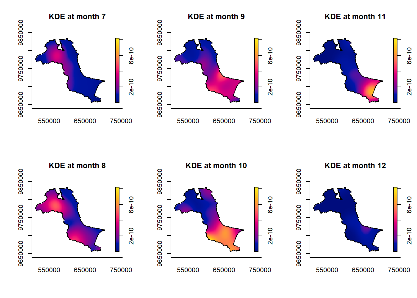
Fraction of frame area: 0.334Computing Spatio-Temporal KDE Next, spattemp.density() of sparr package is used to compute the STKDE
st_kde <- spattemp.density(fire_month_owin)
summary(st_kde)
Spatiotemporal Kernel Density Estimate
Bandwidths
h = 15102.47 (spatial)
lambda = 0.0304 (temporal)
No. of observations
741
Spatial bound
Type: polygonal
2D enclosure: [512066.8, 705559.4] x [9655398, 9834006]
Temporal bound
[1, 12]
Evaluation
128 x 128 x 12 trivariate lattice
Density range: [1.233458e-27, 8.202976e-10]In the code chunk below, plot() of R base is used to get the KDE for between July 2023 - December 2023
tims <- c(7, 8, 9, 10, 11, 12)
par(mfcol=c(2, 3))
for(i in tims){
  plot(st_kde, i,
       override.par=FALSE,
       fix.range=TRUE,
       main=paste("KDE at month", i))
}