pacman::p_load(sf, sfdep, tmap, tidyverse)In Class exercise 6
Analysis
R
sf
tidyverse
6.0 Notes:
Local statistics
Identifying outliers based on a certain attribute of its neighbours
Tobler’s First law of Geography: Everything is related to everything else, but near things are more related than distant things
Geospatial Dependency
- Spatial dependence is the spatial relationship of variable values (for themes defined over space, such as rainfall) or locations (for themes defined as objects, such as cities).
Spatial Autocorrelation
- Spatial autocorrelation is the term used to describe the presence of systematic spatial variation in a variable.
- Inferred after the rejections of the null hypothesis
- Positive autocorrelation: A big lump, congregation of points on the grid
- Negative autocorrelation: More outliers can be seen, checkers board pattern seen
Local Indicator of Spatial Analysis (LISA)
A subset of localised geospatial statistics methods.
Any spatial statistics that satisfies the following two requirements (Anselin, L. 1995):
the LISA for each observation gives an indication of the extent of significant spatial clustering of similar values around that observation;
the sum of LISAs for all observations is proportional to a global indicator of spatial association.
Identify outliers or clusters
6.1 Installing and Loading the R packages
For the purpose of this study, five R packages will be used. They are:
sf, a relatively new R package specially designed to import, manage and process vector-based geospatial data in R.
spatstat, a comprehensive package for point pattern analysis. We’ll use it to perform first- and second-order spatial point pattern analyses and to derive kernel density estimation (KDE) layers.
sfdep, an R package that acts as an interface to ‘spdep’ to integrate with ‘sf’ objects and the ‘tidyverse’.
tidyverse, a collection of R packages designed for data science. It includes packages like
dplyrfor data manipulation,ggplot2for data visualization, andtidyrfor data tidying, all of which are essential for handling and analyzing data efficiently in a clean and consistent manner.
6.1.1 Import shapefile into r environment
The code chunk below uses st_read() of sf package to import Hunan shapefile into R. The imported shapefile will be simple features Object of sf.
hunan_sf <- st_read(dsn = "data/In-class_Ex05/geospatial",
                 layer = "Hunan")
Reading layer `Hunan' from data source
`C:\Users\blzll\OneDrive\Desktop\Y3S1\IS415\Quarto\IS415\In-class_Ex\data\In-class_Ex05\geospatial'
using driver `ESRI Shapefile'
Simple feature collection with 88 features and 7 fields
Geometry type: POLYGON
Dimension: XY
Bounding box: xmin: 108.7831 ymin: 24.6342 xmax: 114.2544 ymax: 30.12812
Geodetic CRS: WGS 846.1.2 Import csv file into r environment
Next, we will import Hunan_2012.csv into R by using read_csv() of readr package. The output is R dataframe class.
hunan2012 <- read_csv("data/In-class_Ex05/aspatial/Hunan_2012.csv")
hunan2012
# A tibble: 88 × 29
County City avg_wage deposite FAI Gov_Rev Gov_Exp GDP GDPPC GIO
<chr> <chr> <dbl> <dbl> <dbl> <dbl> <dbl> <dbl> <dbl> <dbl>
1 Anhua Yiyang 30544 10967 6832. 457. 2703 13225 14567 9277.
2 Anren Chenz… 28058 4599. 6386. 221. 1455. 4941. 12761 4189.
3 Anxiang Chang… 31935 5517. 3541 244. 1780. 12482 23667 5109.
4 Baojing Hunan… 30843 2250 1005. 193. 1379. 4088. 14563 3624.
5 Chaling Zhuzh… 31251 8241. 6508. 620. 1947 11585 20078 9158.
6 Changning Hengy… 28518 10860 7920 770. 2632. 19886 24418 37392
7 Changsha Chang… 54540 24332 33624 5350 7886. 88009 88656 51361
8 Chengbu Shaoy… 28597 2581. 1922. 161. 1192. 2570. 10132 1681.
9 Chenxi Huaih… 33580 4990 5818. 460. 1724. 7755. 17026 6644.
10 Cili Zhang… 33099 8117. 4498. 500. 2306. 11378 18714 5843.
# ℹ 78 more rows
# ℹ 19 more variables: Loan <dbl>, NIPCR <dbl>, Bed <dbl>, Emp <dbl>,
# EmpR <dbl>, EmpRT <dbl>, Pri_Stu <dbl>, Sec_Stu <dbl>, Household <dbl>,
# Household_R <dbl>, NOIP <dbl>, Pop_R <dbl>, RSCG <dbl>, Pop_T <dbl>,
# Agri <dbl>, Service <dbl>, Disp_Inc <dbl>, RORP <dbl>, ROREmp <dbl>6.1.3 Performing relational join
The code chunk below will be used to update the attribute table of hunan’s SpatialPolygonsDataFrame with the attribute fields of hunan2012 data frame. This is performed by using left_join() of dplyr package.
hunan_GDPPC <- left_join(hunan_sf,hunan2012)%>%
  select(1:4, 7, 15)
6.2 Plotting the chloropleth map
Deriving Queen’s contiguity weights: sfdep methods
wm_q <- hunan_GDPPC %>%
  mutate(nb = st_contiguity(geometry),
         wt = st_weights(nb, style = "W"),
         .before = 1)
Computing Global Moran’s I
moranI <- global_moran(wm_q$GDPPC, wm_q$nb, wm_q$wt)
glimpse(moranI)
List of 2
$ I: num 0.301
$ K: num 7.64In general, Moran’s I test will be performed instead of just computing the Moran’s statistics. With sfdep package, Moran’s I test can be performed by using global_moran_test() as shown in the code chunk below:
global_moran_test(wm_q$GDPPC, wm_q$nb, wm_q$wt)
    Moran I test under randomisation

data:  x
weights: listw

Moran I statistic standard deviate = 4.7351, p-value = 1.095e-06
alternative hypothesis: greater
sample estimates:
Moran I statistic       Expectation          Variance
      0.300749970      -0.011494253       0.004348351
Expectation: -0.011494253 negative value suggests clustering
p-value will determine whether the null hypothesis is rejected or not. Not rejecting the null hypothesis would result in the statistic derived from Moran I to be unusable
global_moran_perm(wm_q$GDPPC, wm_q$nb, wm_q$wt, nsim=99)
    Monte-Carlo simulation of Moran I

data:  x
weights: listw
number of simulations + 1: 100

statistic = 0.30075, observed rank = 100, p-value < 2.2e-16
alternative hypothesis: two.sided
As seen from the moran I statistic, even thought the p-value is far smaller, the statistic is stable, approaching 0.30075
set.seed(1234)It is always good to set.seed() before performing simulation, to ensure reproducibility.
lisa <- wm_q %>%
  mutate(local_moran = local_moran(
    GDPPC, nb, wt, nsim = 99),
    .before = 1) %>%
  unnest(local_moran)
To ensure consistency, stay with 1 type of p-value either p_ii, p_ii_sim or p_folded_sim
Mean useful if the data follows the trend of standard distribution and Median would be useful if skewness (close to 0) is detected - Note that row consistency also applies to mean or median - Examine the current trend of the skewness to make these decisions
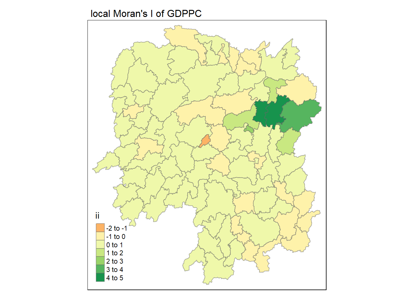
tmap_mode("plot")
tm_shape(lisa) +
  tm_fill("ii") +
  tm_borders(alpha = 0.5) +
  tm_view(set.zoom.limits = c(6,8)) +
  tm_layout(
    main.title = "local Moran's I of GDPPC",
    main.title.size = 1
  )
tmap_mode("plot")
map1 <- tm_shape(lisa) +
  tm_fill("ii") +
  tm_borders(alpha = 0.5) +
  tm_view(set.zoom.limits = c(6,8)) +
  tm_layout(
    main.title = "local Moran's I of GDPPC",
    main.title.size = 1
  )

map2 <- tm_shape(lisa) +
  tm_fill("p_ii", breaks = c(0, 0.001, 0.01, 0.05, 1),
          labels = c("0.001", "0.01", "0.05", "Not sig")) +
  tm_borders(alpha = 0.5) +
  tm_layout(
    main.title = "p-value of local Moran's I",
    main.title.size = 0.8
  )

tmap_arrange(map1, map2, ncol = 2)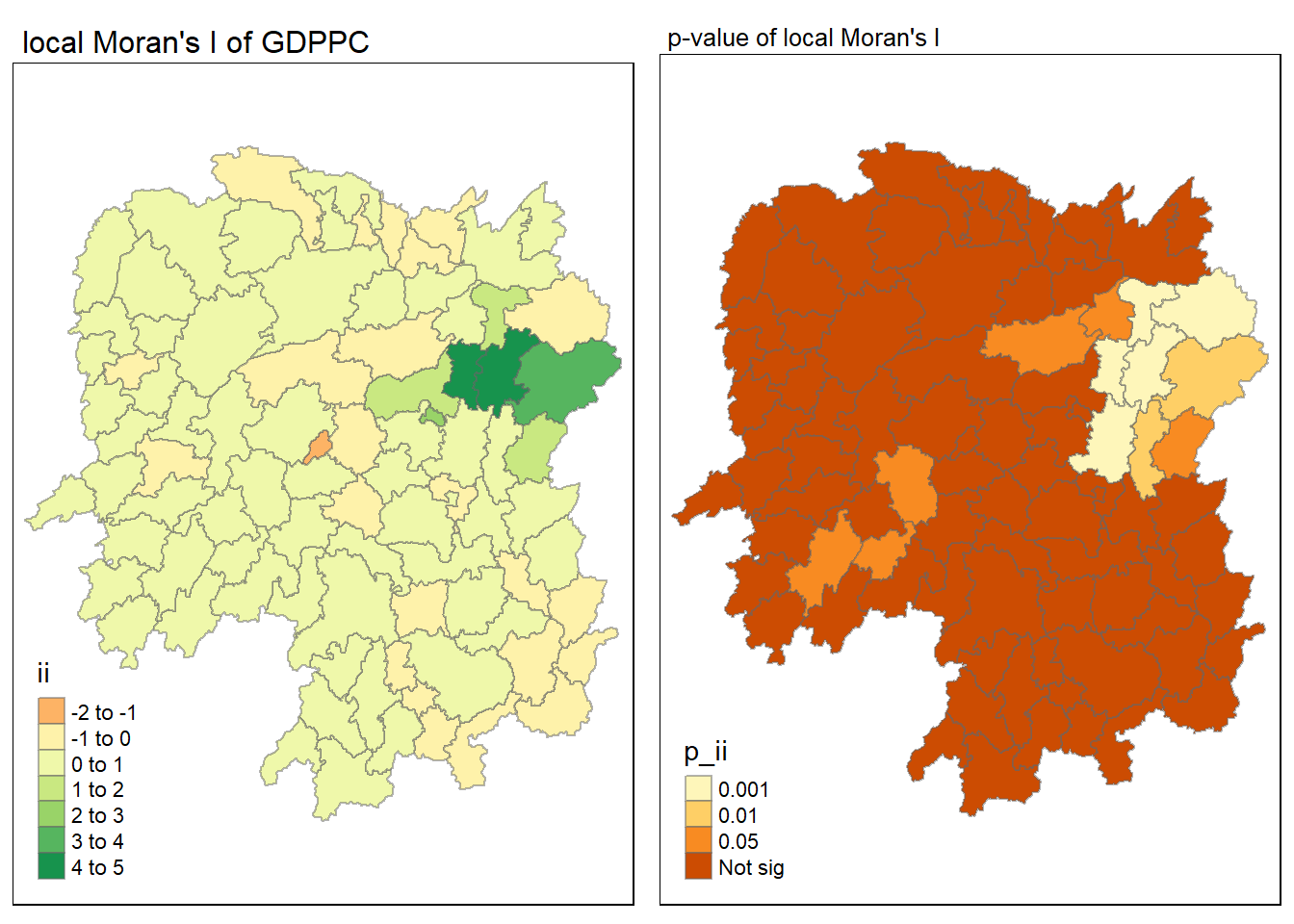
Visualising LISA map
lisa_sig <- lisa %>%
  filter(p_ii < 0.05)
tmap_mode("plot")
tm_shape(lisa) +
  tm_polygons() +
  tm_borders(alpha = 0.5) +
tm_shape(lisa_sig) +
  tm_fill("mean") +
  tm_borders(alpha = 0.4)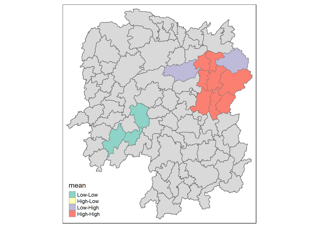
LISA map is categorical map showing outliers and clusters. There are two types of outliers namely: High-Low and Low-High outliers. Likewise, there are two types of clusters namely: High-High and Low-Low
Computing local Gi* statistics
As usual we will need to derive a spatial weight matrix before we can compute local Gi* statistics. Code chunk below will be used to derive a spatial weight matrix by using sfdep functions and tidyverse approach.
wm_idw <- hunan_GDPPC %>%
  mutate(nb = st_contiguity(geometry),
         wts = st_inverse_distance(nb, geometry,
                                   scale = 1,
                                   alpha = 1),
         .before = 1)
Calculating the local Gi* by using the code chunk below:
HCSA <- wm_idw %>%
  mutate(local_Gi = local_gstar_perm(
    GDPPC, nb, wt, nsim = 99),
         .before = 1) %>%
  unnest(local_Gi)
HCSA
Simple feature collection with 88 features and 18 fields
Geometry type: POLYGON
Dimension: XY
Bounding box: xmin: 108.7831 ymin: 24.6342 xmax: 114.2544 ymax: 30.12812
Geodetic CRS: WGS 84
# A tibble: 88 × 19
gi_star cluster e_gi var_gi std_dev p_value p_sim p_folded_sim skewness
<dbl> <fct> <dbl> <dbl> <dbl> <dbl> <dbl> <dbl> <dbl>
1 0.0416 Low 0.0114 0.00000721 0.0376 9.70e-1 0.8 0.4 0.901
2 -0.333 Low 0.0111 0.00000553 -0.299 7.65e-1 0.92 0.46 0.941
3 0.281 High 0.0121 0.00000832 0.0405 9.68e-1 0.8 0.4 0.912
4 0.411 High 0.0117 0.00000943 0.298 7.66e-1 0.68 0.34 1.09
5 0.387 High 0.0113 0.00000869 0.415 6.78e-1 0.5 0.25 0.992
6 -0.368 High 0.0116 0.00000605 -0.498 6.18e-1 0.76 0.38 1.15
7 3.56 High 0.0149 0.00000745 2.67 7.56e-3 0.04 0.02 0.950
8 2.52 High 0.0135 0.00000482 1.74 8.17e-2 0.14 0.07 0.434
9 4.56 High 0.0144 0.00000514 3.77 1.64e-4 0.02 0.01 0.634
10 1.16 Low 0.0108 0.00000479 1.45 1.48e-1 0.18 0.09 0.476
# ℹ 78 more rows
# ℹ 10 more variables: kurtosis <dbl>, nb <nb>, wts <list>, NAME_2 <chr>,
# ID_3 <int>, NAME_3 <chr>, ENGTYPE_3 <chr>, County <chr>, GDPPC <dbl>,
# geometry <POLYGON [°]>Visualising hot spot and cold spot areas
Show the code
tmap_mode("plot")
map1 <- tm_shape(HCSA) +
  tm_fill("gi_star") +
  tm_borders(alpha = 0.5) +
  tm_view(set.zoom.limits = c(6,8)) +
  tm_layout(main.title = "Gi* of GDPPC",
            main.title.size = 0.8)

map2 <- tm_shape(HCSA) +
  tm_fill("p_value",
          breaks = c(0, 0.001, 0.01, 0.05, 1),
              labels = c("0.001", "0.01", "0.05", "Not sig")) +
  tm_borders(alpha = 0.5) +
  tm_layout(main.title = "p-value of Gi*",
            main.title.size = 0.8)

tmap_arrange(map1, map2, ncol = 2)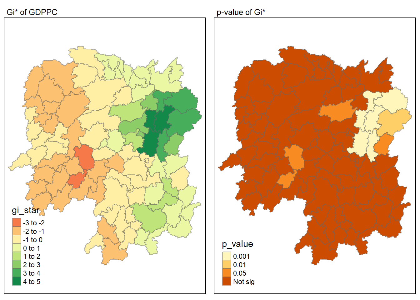
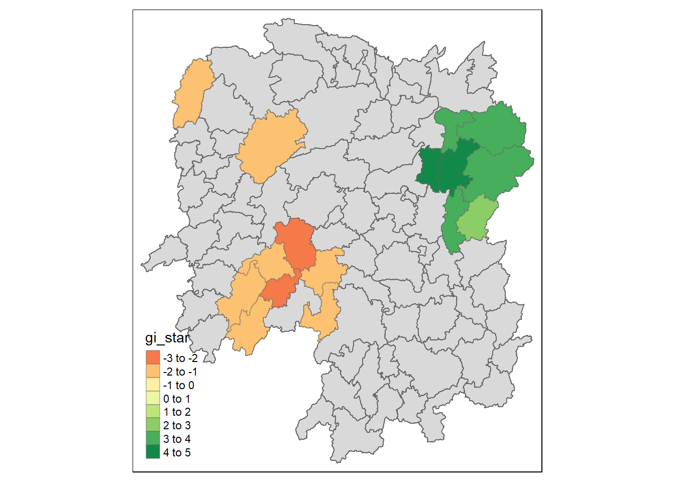
HCSA_sig <- HCSA %>%
  filter(p_sim < 0.05)
tmap_mode("plot")
tm_shape(HCSA) +
  tm_polygons() +
  tm_borders(alpha = 0.5) +
  tm_shape(HCSA_sig) +
  tm_fill("gi_star") +
  tm_borders(alpha = 0.4)