In Class exercise 10

6.0 Loading the R packages

pacman::p_load(spdep, sp, tmap, sf, ClustGeo, cluster, factoextra, NbClust, tidyverse, GGally)

shan_sf <- read_rds("data/In-class_Ex09/rds/shan_sf.rds")
shan_ict <- read_rds("data/In-class_Ex09/rds/shan_ict.rds")
shan_sf_cluster <- read_rds("data/In-class_Ex09/rds/shan_sf_cluster.rds")

6.1 Conventional Hierarchical Clustering

In R, many packages provide functions to calculate distance matrix. We will compute the proximity matrix by using dist() of R.

dist() supports six distance proximity calculations, they are: euclidean, maximum, manhattan, canberra, binary and minkowski. The default is euclidean proximity matrix.

The code chunk below is used to compute the proximity matrix using euclidean method.

proxmat <- dist(shan_ict, method = "euclidean")
hclust_ward <- hclust(proxmat, method = "ward.D")
groups <- as.factor(cutree(hclust_ward, k=6))

hclust() will take the proximity matrix to perform hierarchical clustering to create a hierarchical clustering object to get the the groups based on the cutree( method

This chunk of code is meant to tidy the shan_sf_cluster dataset

shan_sf_cluster <- cbind(shan_sf, as.matrix(groups)) %>%
  rename(`CLUSTER`=`as.matrix.groups.`) %>%
  select(-c(3:4, 7:9)) %>%
  rename(TS = TS.x)

This chunk of code to create the dendogram

plot(hclust_ward, cex = 0.6)
rect.hclust(hclust_ward, k = 6, border = 2.5)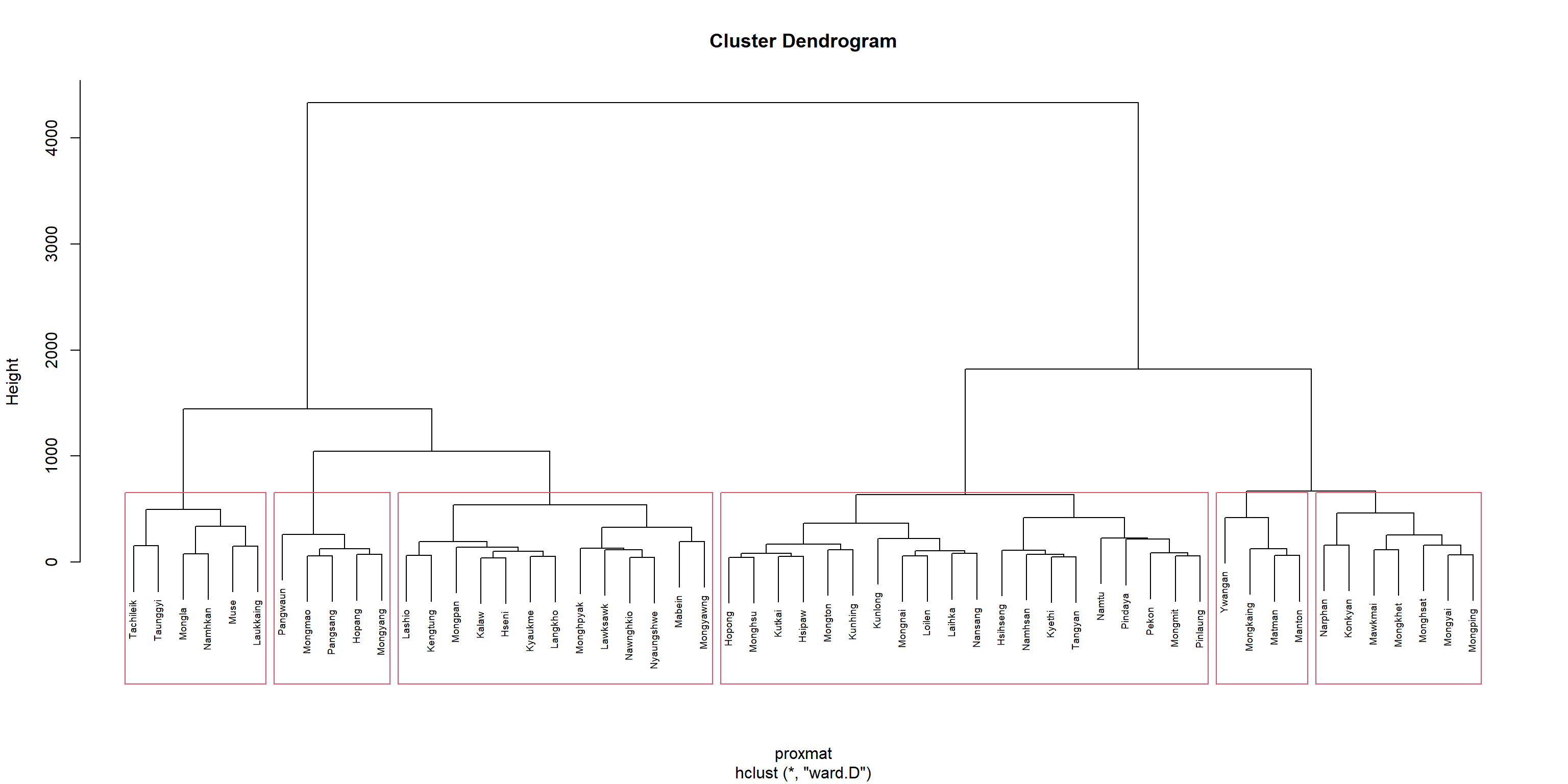

This chunk of code to create the cluster map of the shan_sf_cluster object

qtm(shan_sf_cluster, "CLUSTER")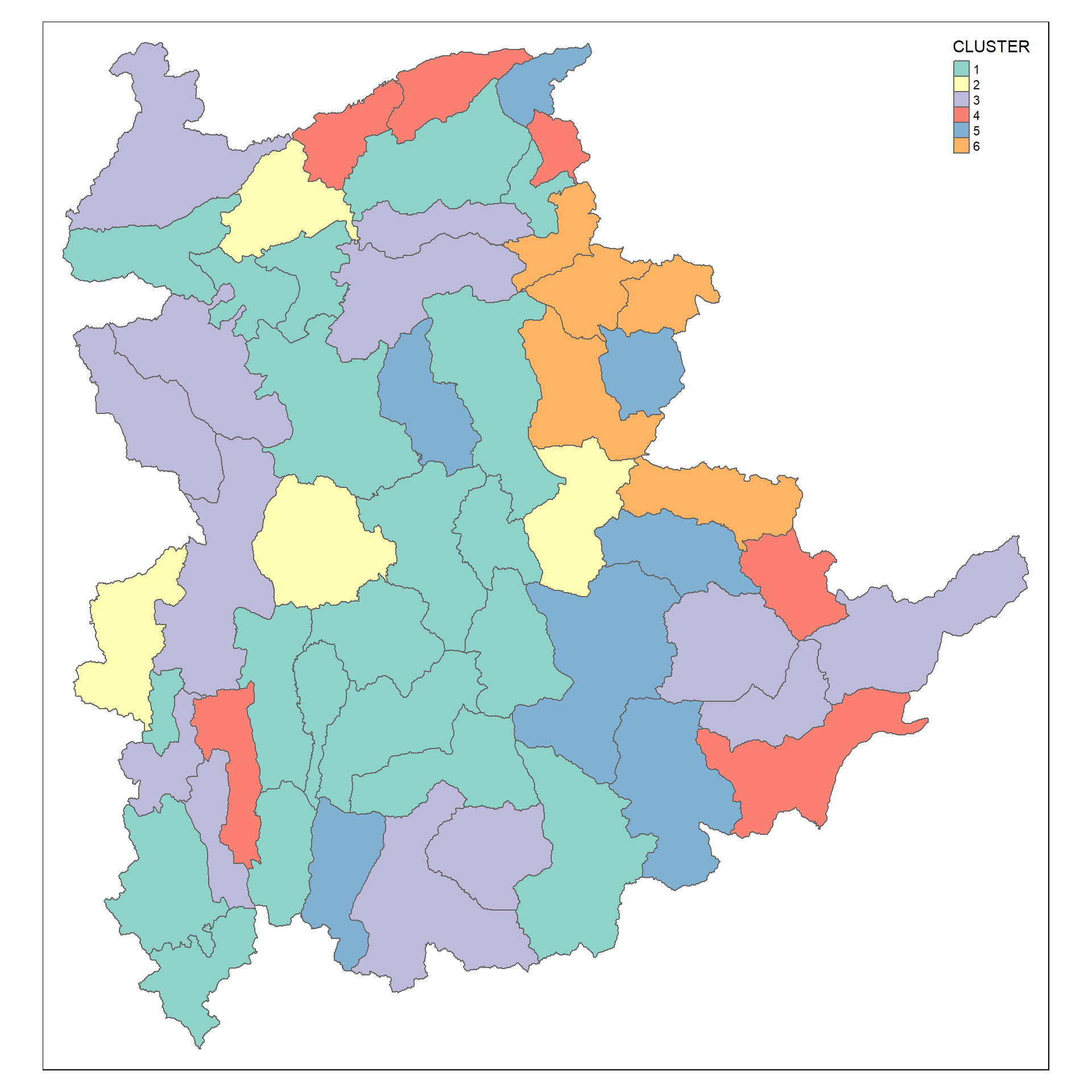

Spatially Constrained Clustering

• SKATER (Spatial ’K’luser Analysis by Tree Edge Removal) Alogrithm

• REDCAP (Reorganisation with dynamically

• ClustGeo Algorithm

SKATER Algorithm

Spatially Constrained Clustering: SKATER Method

1. Computing nearest neighbours (Minimum Spanning Tree)

shan.nb <- poly2nb(shan_sf)
summary(shan.nb)

Neighbour list object:
Number of regions: 55 
Number of nonzero links: 264 
Percentage nonzero weights: 8.727273 
Average number of links: 4.8 
Link number distribution:

 2  3  4  5  6  7  8  9 
 5  9  7 21  4  3  5  1 
5 least connected regions:
3 5 7 9 47 with 2 links
1 most connected region:
8 with 9 links

2. Visualising the neighbours

plot(st_geometry(shan_sf),
     border=grey(.5))
pts <- st_coordinates(st_centroid(shan_sf))
plot(shan.nb, pts, col="blue", add=TRUE)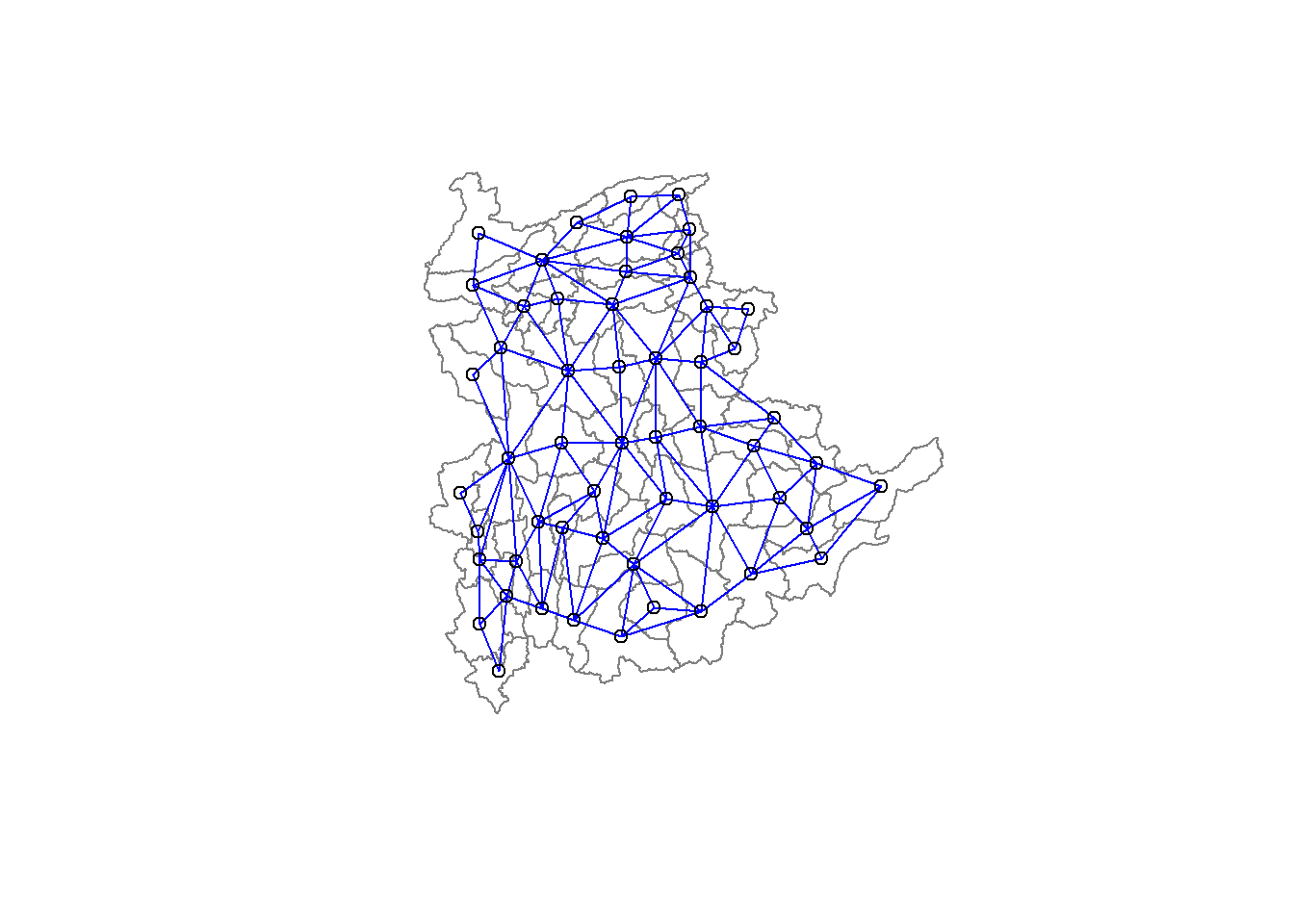

3. Computing minimum spanning tree (MST)

• Calculating edge costs

lcosts <- nbcosts(shan.nb, shan_ict)

• Incorporating these costs into a weights object

shan.w <- nb2listw(shan.nb, lcosts, style = "B")

summary(shan.w)

Characteristics of weights list object:
Neighbour list object:
Number of regions: 55 
Number of nonzero links: 264 
Percentage nonzero weights: 8.727273 
Average number of links: 4.8 
Link number distribution:

 2  3  4  5  6  7  8  9 
 5  9  7 21  4  3  5  1 
5 least connected regions:
3 5 7 9 47 with 2 links
1 most connected region:
8 with 9 links

Weights style: B 
Weights constants summary:
   n   nn       S0       S1        S2
B 55 3025 76267.65 58260785 522016004

• Visualising MST

shan.mst <- mstree(shan.w)

plot(st_geometry(shan_sf), border=gray(.5))
plot.mst(shan.mst, 
         pts, 
         col="blue", 
         cex.lab=0.7, 
         cex.circles = 0.005, 
         add=TRUE)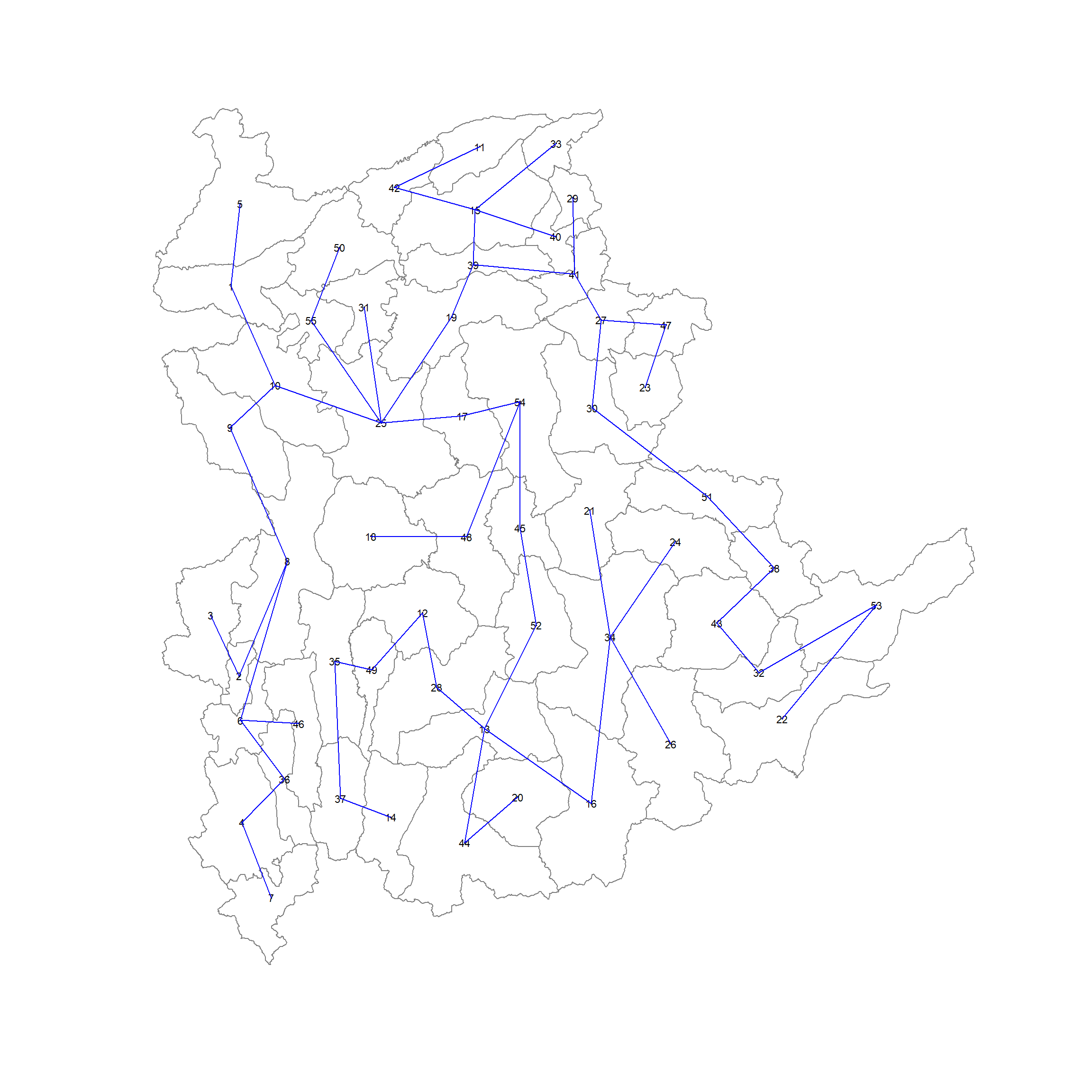

Computing spatially constrained clusters using SKATER method

skater.clust6 <- skater(edges = shan.mst[,1:2],
                        data = shan_ict,
                        method = "euclidean",
                        ncuts = 5)

The following code chunk plots the skater tree

plot(st_geometry(shan_sf), border=gray(.5))
plot(skater.clust6, 
         pts, 
         cex.lab=.7,
         groups.colors=c("red", "green", "blue", "brown", "pink"),
         cex.circles = 0.005, 
         add=TRUE)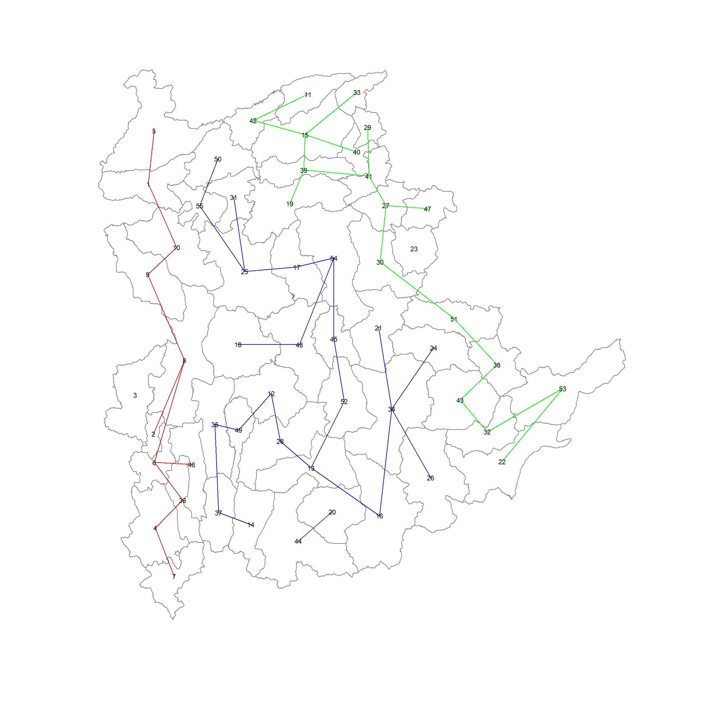

Visualising clusters in chloropeth map

groups_mat<- as.matrix(skater.clust6$groups)
shan_sf_spatialcluster <- cbind(shan_sf_cluster, as.factor(groups_mat)) %>%
  rename(`skater_CLUSTER` = `as.factor.groups_mat.`)
qtm(shan_sf_spatialcluster, "skater_CLUSTER")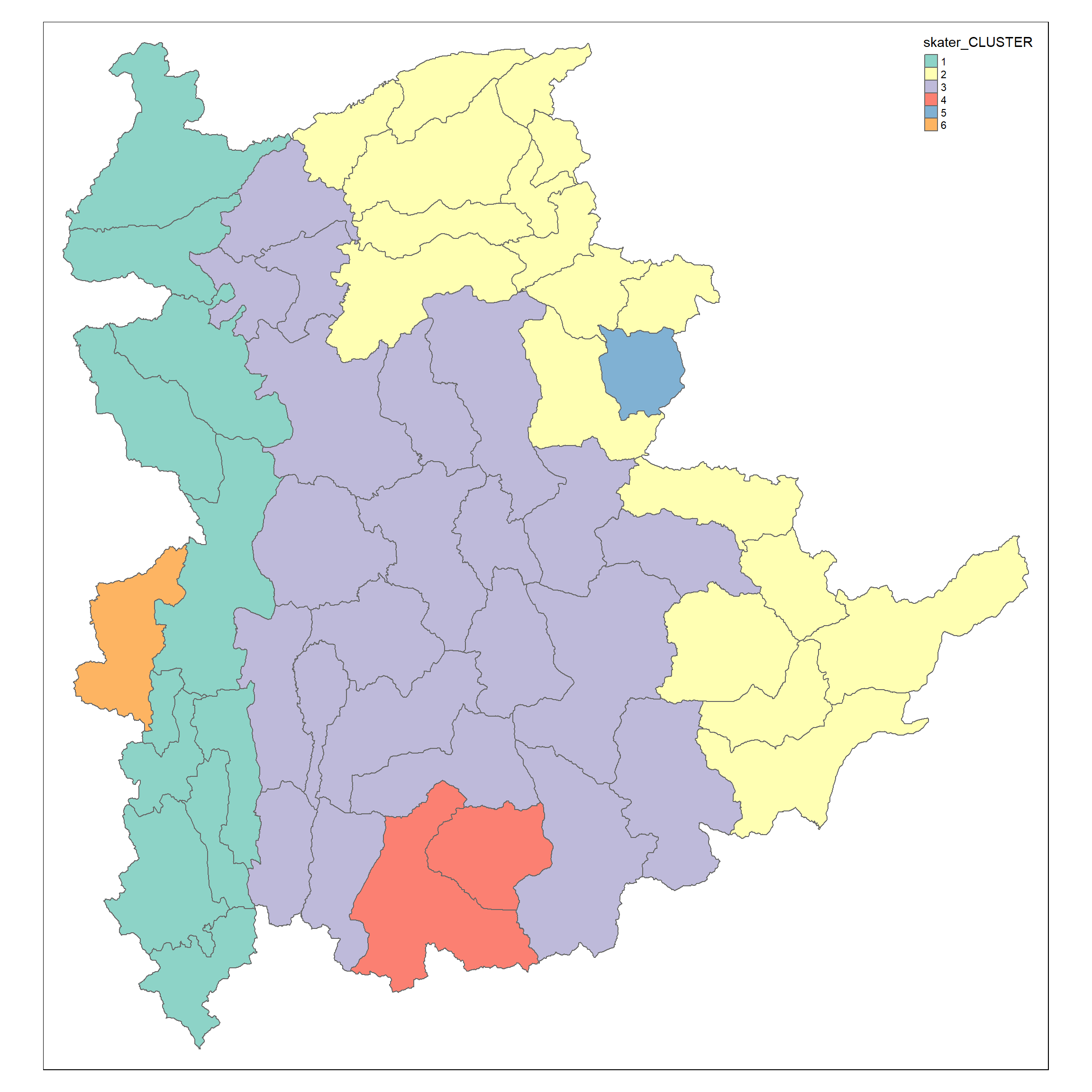

ClustGeo Algoritm

1. Compute Spatial Distance Matrix To compute the distance matrix using st_distance() of sf package.

dist <- st_distance(shan_sf, shan_sf)
distmat <- as.dist(dist)

2. Cluster Graph

cr <- choicealpha(proxmat, distmat, 
                  range.alpha = seq(0, 1, 0.1), 
                  K=6, graph = TRUE)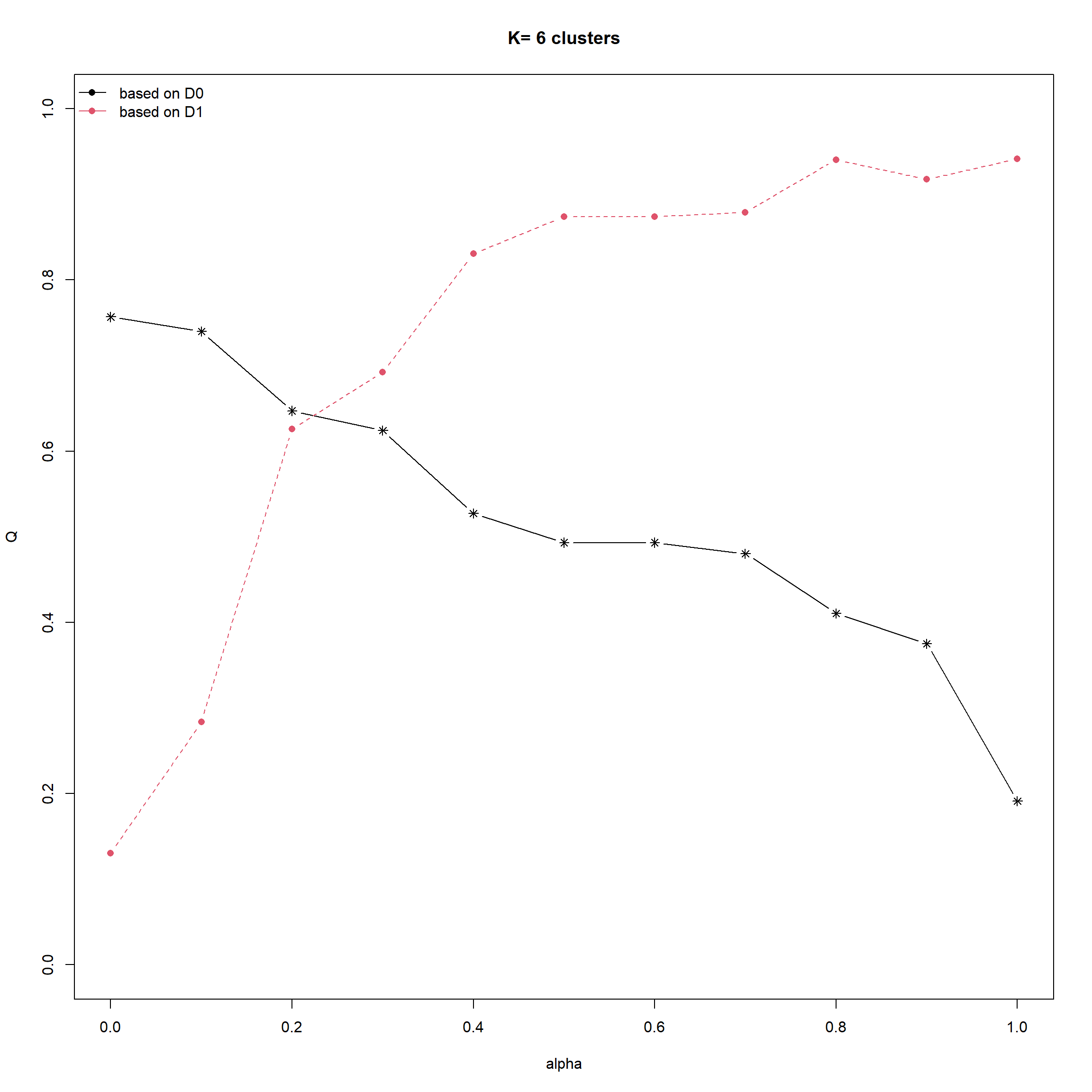

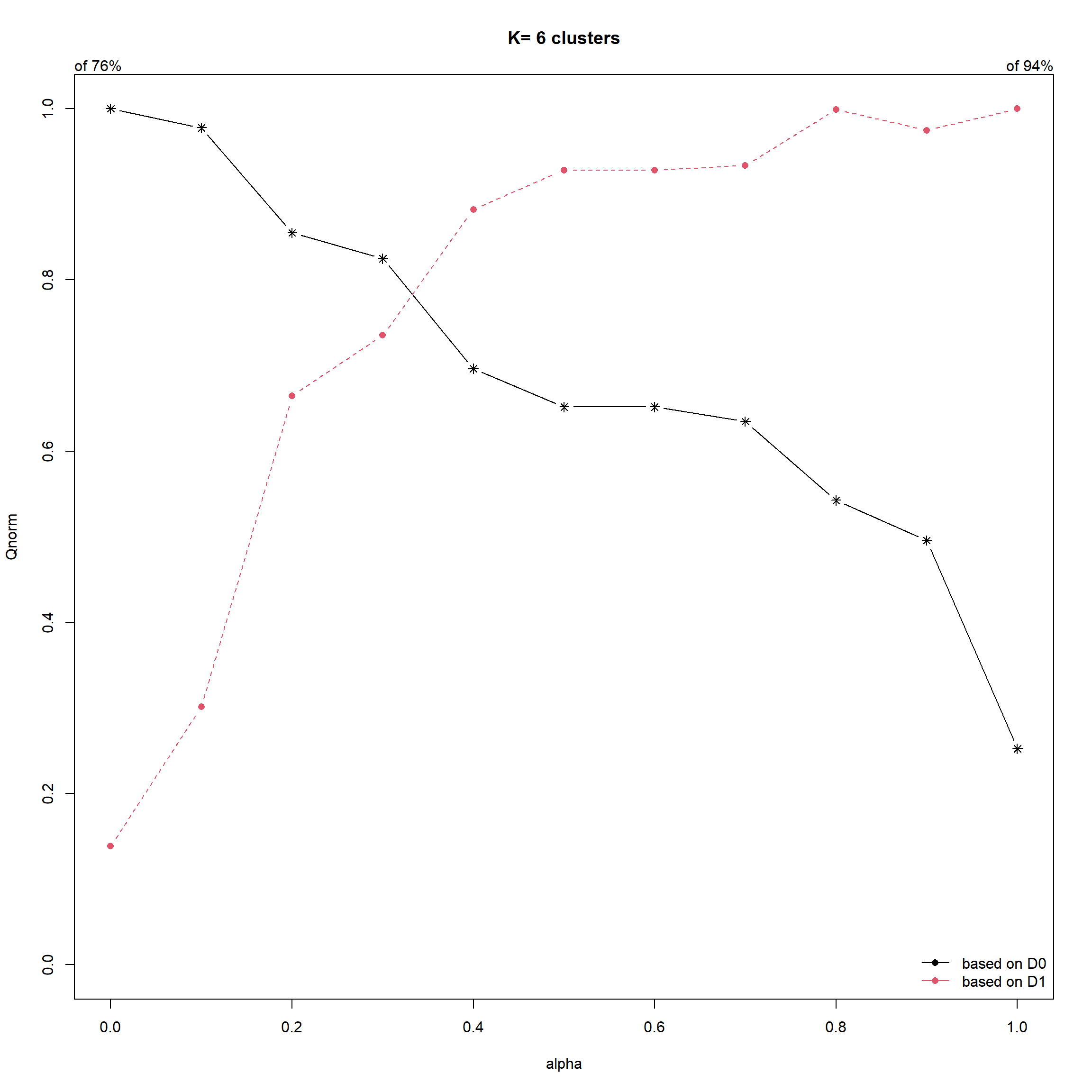
3. Saving ClustGeo Output

clustG <- hclustgeo(proxmat, distmat, alpha = 0.2)
groups <- as.factor(cutree(clustG, k=6))
shan_sf_GclusterGeo <- cbind(shan_sf, as.matrix(groups)) %>%
  rename(`clustGeo` = `as.matrix.groups.`)

qtm(shan_sf_GclusterGeo, "clustGeo")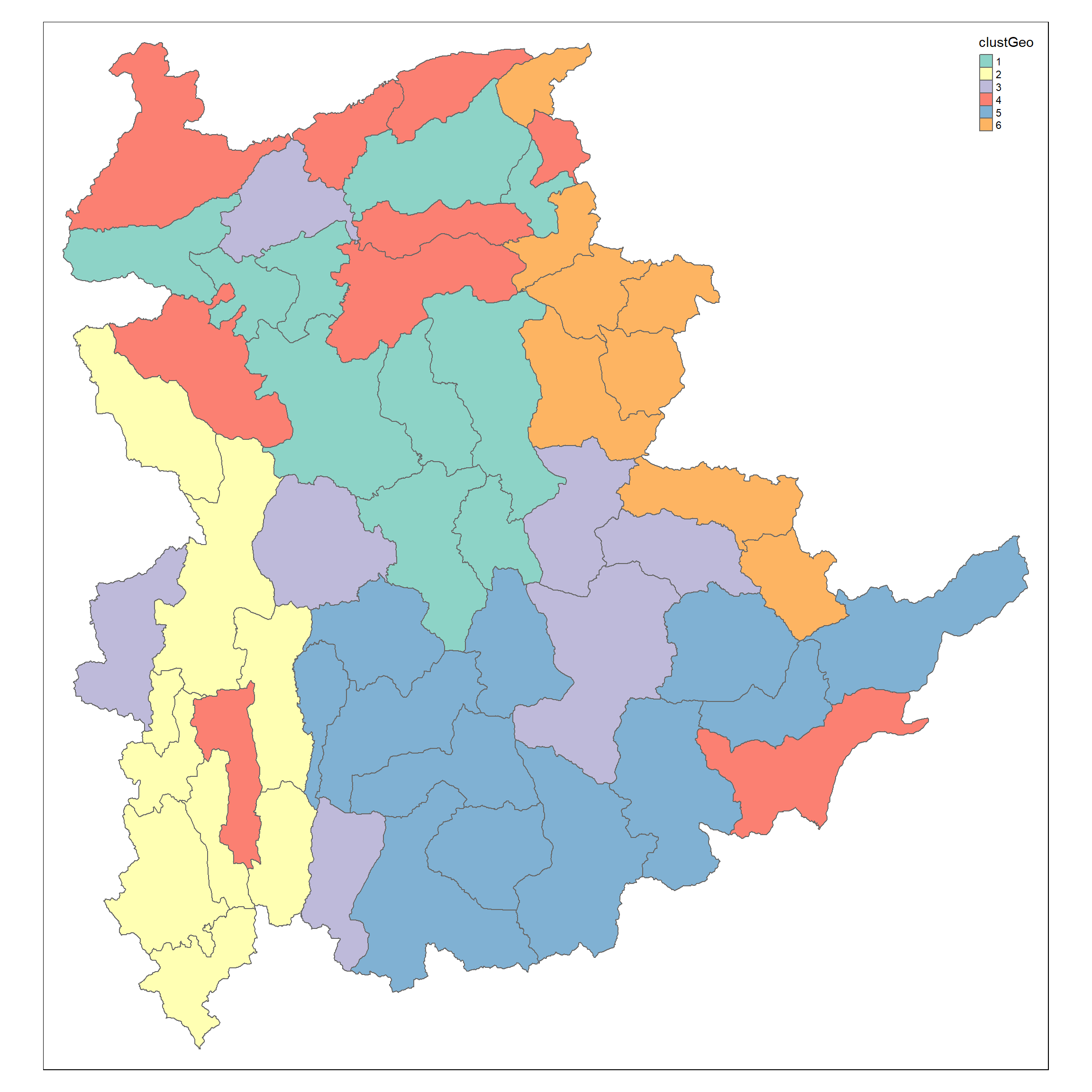

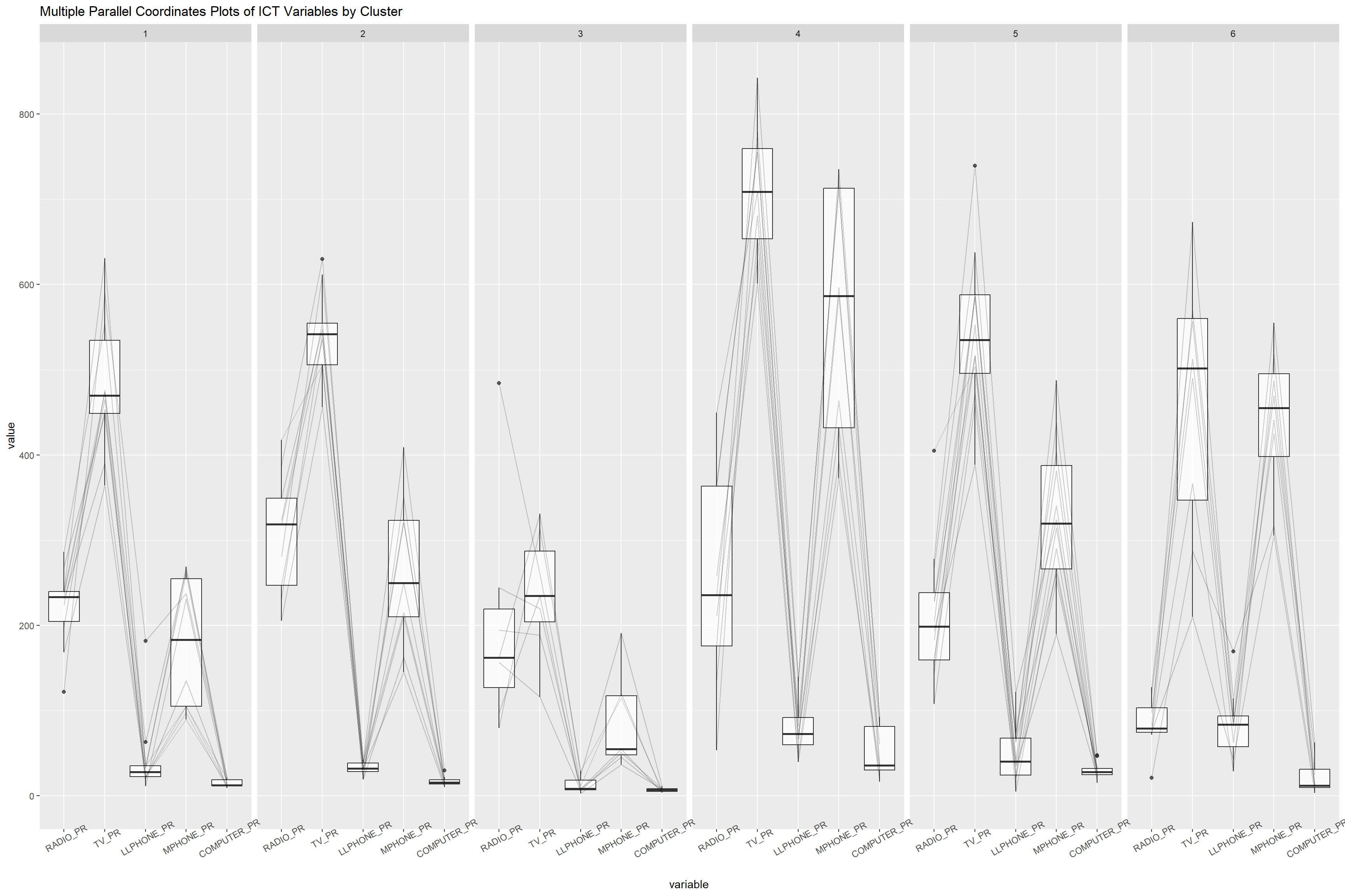
4. Characterising the Clusters

ggparcoord(data = shan_sf_GclusterGeo, 
           columns = c(17:21), 
           scale = "globalminmax",
           alphaLines = 0.2,
           boxplot = TRUE, 
           title = "Multiple Parallel Coordinates Plots of ICT Variables by Cluster") +
  facet_grid(~ clustGeo) + 
  theme(axis.text.x = element_text(angle = 30))