pacman::p_load(
  olsrr,
  ggstatsplot,
  corrplot,
  ggpubr,
  sfdep,
  sf,
  spdep,
  GWmodel,
  tmap,
  tidyverse,
  performance,
  see
)In Class exercise 11
Analysis
R
sf
tidyverse
cluster
ClustGeo
NbClust
GGally
Note
Explanatory vs Predictive modeling
Explanatory model => aims to identify factors/independent variable that are causally related to an outcome.
- Hedonic Pricing Model using GWmodel
Predictive model => aims to find the combination of factors that best predicts the dependent variable.
- Calibrating Random Forest Model
R-square VS Adj R-Square => Adj R-Square account for the number of predictors in the model, providing a more accurate measure of fit.
Regression Diagnostics
Multicollinearity
VIF
Below than 5: lower multicollinearity
More than 5 and Below 10: Moderate multicolinearity
More than 10: Strong multicolinearity
Make use of the correlation matrix to determine the pairs and drop one of them if their VIF is high.
Linearity Assumption
- The relationship between X and the mean of Y is linear or not.
Normality Assumption
- Check if the residual is normally distributed
Spatial Autocorrelation
- Use Moran’s I test to check the residual spatial autocorrelation
Loading the R packages
Importing the Data
mpsz = st_read(dsn = "data/MasterPlan2014SubzoneBoundaryWebSHP", layer = "MP14_SUBZONE_WEB_PL")Reading layer `MP14_SUBZONE_WEB_PL' from data source
`C:\Users\blzll\OneDrive\Desktop\Y3S1\IS415\Quarto\IS415\In-class_Ex\data\MasterPlan2014SubzoneBoundaryWebSHP'
using driver `ESRI Shapefile'
Simple feature collection with 323 features and 15 fields
Geometry type: MULTIPOLYGON
Dimension: XY
Bounding box: xmin: 2667.538 ymin: 15748.72 xmax: 56396.44 ymax: 50256.33
Projected CRS: SVY21mpsz_svy21 <- st_transform(mpsz, 3414)
condo_resale = read_csv("data/In-class_Ex11/aspatial/Condo_resale_2015.csv")
condo_resale_sf <- st_as_sf(condo_resale,
coords = c("LONGITUDE", "LATITUDE"),
crs=4326) %>%
st_transform(crs=3414)Correlation Analysis - ggstatsplot methods
ggcorrmat(condo_resale[,5:23])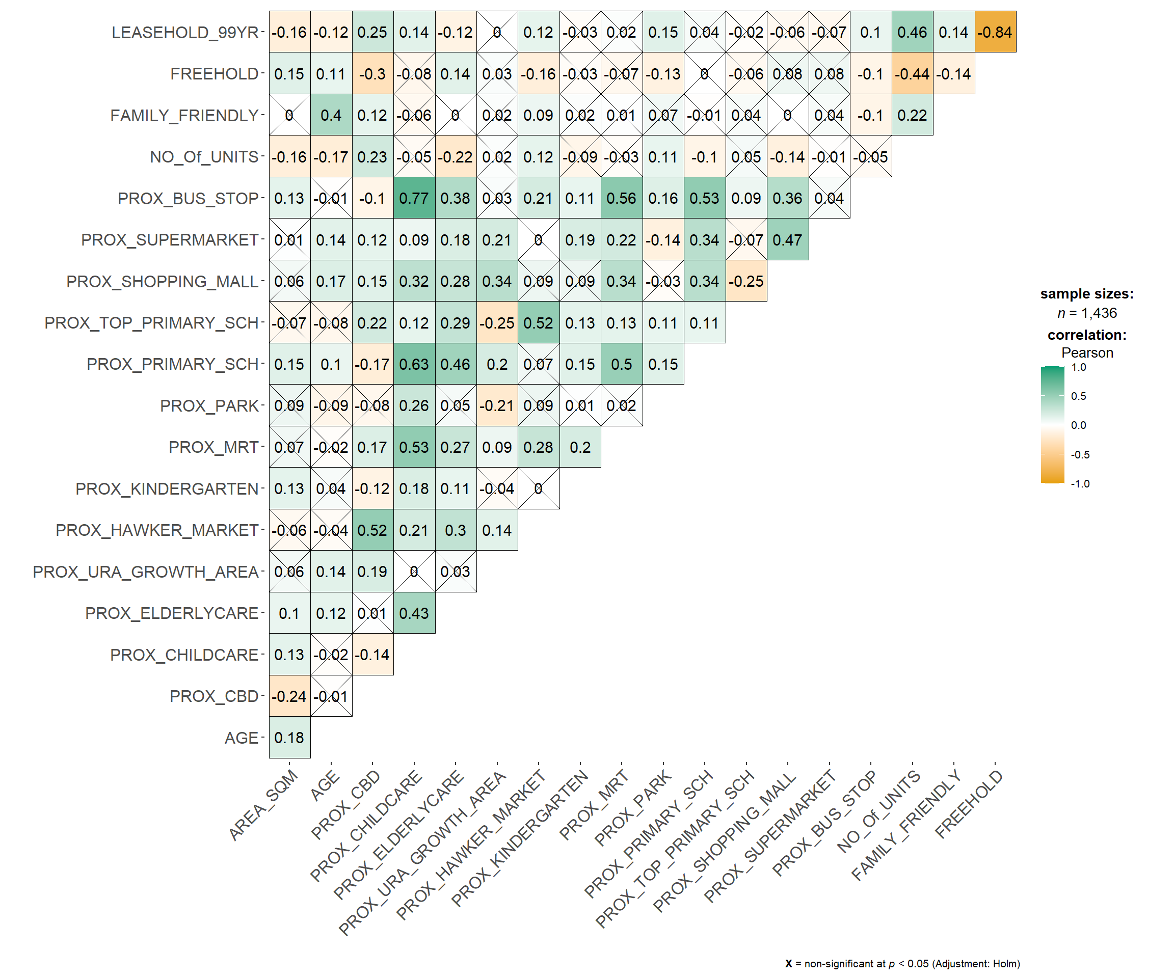
Building a Hedonic Pricing Model by using Multiple Linear Regression Method
condo_mlr <- lm(formula = SELLING_PRICE ~ AREA_SQM + AGE    +
                  PROX_CBD + PROX_CHILDCARE + PROX_ELDERLYCARE +
                  PROX_URA_GROWTH_AREA + PROX_HAWKER_MARKET + PROX_KINDERGARTEN +
                  PROX_MRT  + PROX_PARK + PROX_PRIMARY_SCH +
                  PROX_TOP_PRIMARY_SCH + PROX_SHOPPING_MALL + PROX_SUPERMARKET +
                  PROX_BUS_STOP + NO_Of_UNITS + FAMILY_FRIENDLY + FREEHOLD,
                data=condo_resale_sf)
summary(condo_mlr)
Call:
lm(formula = SELLING_PRICE ~ AREA_SQM + AGE + PROX_CBD + PROX_CHILDCARE +
    PROX_ELDERLYCARE + PROX_URA_GROWTH_AREA + PROX_HAWKER_MARKET +
    PROX_KINDERGARTEN + PROX_MRT + PROX_PARK + PROX_PRIMARY_SCH +
    PROX_TOP_PRIMARY_SCH + PROX_SHOPPING_MALL + PROX_SUPERMARKET +
    PROX_BUS_STOP + NO_Of_UNITS + FAMILY_FRIENDLY + FREEHOLD,
    data = condo_resale_sf)

Residuals:
     Min       1Q   Median       3Q      Max
-3475964  -293923   -23069   241043 12260381

Coefficients:
                       Estimate Std. Error t value Pr(>|t|)
(Intercept)           481728.40  121441.01   3.967 7.65e-05 ***
AREA_SQM               12708.32     369.59  34.385  < 2e-16 ***
AGE                   -24440.82    2763.16  -8.845  < 2e-16 ***
PROX_CBD              -78669.78    6768.97 -11.622  < 2e-16 ***
PROX_CHILDCARE       -351617.91  109467.25  -3.212  0.00135 **
PROX_ELDERLYCARE      171029.42   42110.51   4.061 5.14e-05 ***
PROX_URA_GROWTH_AREA   38474.53   12523.57   3.072  0.00217 **
PROX_HAWKER_MARKET     23746.10   29299.76   0.810  0.41782
PROX_KINDERGARTEN     147468.99   82668.87   1.784  0.07466 .
PROX_MRT             -314599.68   57947.44  -5.429 6.66e-08 ***
PROX_PARK             563280.50   66551.68   8.464  < 2e-16 ***
PROX_PRIMARY_SCH      180186.08   65237.95   2.762  0.00582 **
PROX_TOP_PRIMARY_SCH    2280.04   20410.43   0.112  0.91107
PROX_SHOPPING_MALL   -206604.06   42840.60  -4.823 1.57e-06 ***
PROX_SUPERMARKET      -44991.80   77082.64  -0.584  0.55953
PROX_BUS_STOP         683121.35  138353.28   4.938 8.85e-07 ***
NO_Of_UNITS             -231.18      89.03  -2.597  0.00951 **
FAMILY_FRIENDLY       140340.77   47020.55   2.985  0.00289 **
FREEHOLD              359913.01   49220.22   7.312 4.38e-13 ***
---
Signif. codes:  0 '***' 0.001 '**' 0.01 '*' 0.05 '.' 0.1 ' ' 1

Residual standard error: 755800 on 1417 degrees of freedom
Multiple R-squared:  0.6518,    Adjusted R-squared:  0.6474
F-statistic: 147.4 on 18 and 1417 DF,  p-value: < 2.2e-16
Generating Tidy Linear Regression Report
ols_regress(condo_mlr) Model Summary
-----------------------------------------------------------------------------
R 0.807 RMSE 750799.558
R-Squared 0.652 MSE 571258408962.149
Adj. R-Squared 0.647 Coef. Var 43.160
Pred R-Squared 0.637 AIC 42970.175
MAE 413425.809 SBC 43075.567
-----------------------------------------------------------------------------
RMSE: Root Mean Square Error
MSE: Mean Square Error
MAE: Mean Absolute Error
AIC: Akaike Information Criteria
SBC: Schwarz Bayesian Criteria
ANOVA
--------------------------------------------------------------------------------
Sum of
Squares DF Mean Square F Sig.
--------------------------------------------------------------------------------
Regression 1.515174e+15 18 8.417631e+13 147.352 0.0000
Residual 8.094732e+14 1417 571258408962.149
Total 2.324647e+15 1435
--------------------------------------------------------------------------------
Parameter Estimates
-----------------------------------------------------------------------------------------------------------------
model Beta Std. Error Std. Beta t Sig lower upper
-----------------------------------------------------------------------------------------------------------------
(Intercept) 481728.405 121441.014 3.967 0.000 243504.909 719951.900
AREA_SQM 12708.324 369.590 0.580 34.385 0.000 11983.322 13433.326
AGE -24440.816 2763.164 -0.165 -8.845 0.000 -29861.148 -19020.484
PROX_CBD -78669.779 6768.972 -0.268 -11.622 0.000 -91948.061 -65391.496
PROX_CHILDCARE -351617.910 109467.252 -0.092 -3.212 0.001 -566353.201 -136882.619
PROX_ELDERLYCARE 171029.418 42110.506 0.083 4.061 0.000 88423.783 253635.053
PROX_URA_GROWTH_AREA 38474.534 12523.567 0.059 3.072 0.002 13907.809 63041.258
PROX_HAWKER_MARKET 23746.098 29299.755 0.019 0.810 0.418 -33729.461 81221.657
PROX_KINDERGARTEN 147468.986 82668.868 0.031 1.784 0.075 -14697.534 309635.506
PROX_MRT -314599.679 57947.441 -0.120 -5.429 0.000 -428271.672 -200927.687
PROX_PARK 563280.499 66551.675 0.148 8.464 0.000 432730.102 693830.897
PROX_PRIMARY_SCH 180186.083 65237.948 0.070 2.762 0.006 52212.744 308159.421
PROX_TOP_PRIMARY_SCH 2280.036 20410.435 0.002 0.112 0.911 -37757.880 42317.951
PROX_SHOPPING_MALL -206604.057 42840.595 -0.108 -4.823 0.000 -290641.863 -122566.252
PROX_SUPERMARKET -44991.803 77082.635 -0.012 -0.584 0.560 -196200.149 106216.542
PROX_BUS_STOP 683121.347 138353.278 0.134 4.938 0.000 411722.087 954520.608
NO_Of_UNITS -231.180 89.033 -0.050 -2.597 0.010 -405.830 -56.530
FAMILY_FRIENDLY 140340.770 47020.551 0.055 2.985 0.003 48103.399 232578.141
FREEHOLD 359913.008 49220.224 0.140 7.312 0.000 263360.671 456465.345
-----------------------------------------------------------------------------------------------------------------Variable Selection
Forward
condo_fw_mlr <- ols_step_forward_p(
  condo_mlr,
  p_val = 0.05,
  details = FALSE
)
condo_fw_mlr
                                     Stepwise Summary
-----------------------------------------------------------------------------------------
Step    Variable                   AIC          SBC         SBIC         R2       Adj. R2
-----------------------------------------------------------------------------------------
 0      Base Model              44449.068    44459.608    40371.745    0.00000    0.00000
 1      AREA_SQM                43587.753    43603.562    39510.883    0.45184    0.45146
 2      PROX_CBD                43243.523    43264.602    39167.182    0.56928    0.56868
 3      PROX_PARK               43177.691    43204.039    39101.331    0.58915    0.58829
 4      FREEHOLD                43125.474    43157.092    39049.179    0.60438    0.60327
 5      AGE                     43069.222    43106.109    38993.167    0.62010    0.61878
 6      PROX_ELDERLYCARE        43046.515    43088.672    38970.548    0.62659    0.62502
 7      PROX_SHOPPING_MALL      43020.990    43068.417    38945.209    0.63367    0.63188
 8      PROX_URA_GROWTH_AREA    43009.092    43061.788    38933.407    0.63720    0.63517
 9      PROX_MRT                42999.058    43057.024    38923.483    0.64023    0.63796
 10     PROX_BUS_STOP           42984.951    43048.186    38909.581    0.64424    0.64175
 11     FAMILY_FRIENDLY         42981.085    43049.590    38905.797    0.64569    0.64296
 12     NO_Of_UNITS             42975.246    43049.021    38900.092    0.64762    0.64465
 13     PROX_CHILDCARE          42971.858    43050.902    38896.812    0.64894    0.64573
 14     PROX_PRIMARY_SCH        42966.758    43051.072    38891.872    0.65067    0.64723
-----------------------------------------------------------------------------------------

Final Model Output
------------------

                                Model Summary
-----------------------------------------------------------------------------
R                            0.807       RMSE                     751998.679
R-Squared                    0.651       MSE                571471422208.591
Adj. R-Squared               0.647       Coef. Var                    43.168
Pred R-Squared               0.638       AIC                       42966.758
MAE                     414819.628       SBC                       43051.072
-----------------------------------------------------------------------------
 RMSE: Root Mean Square Error
 MSE: Mean Square Error
 MAE: Mean Absolute Error
 AIC: Akaike Information Criteria
 SBC: Schwarz Bayesian Criteria

                                     ANOVA
--------------------------------------------------------------------------------
                    Sum of
                   Squares          DF         Mean Square       F         Sig.
--------------------------------------------------------------------------------
Regression    1.512586e+15          14        1.080418e+14    189.059    0.0000
Residual      8.120609e+14        1421    571471422208.591
Total         2.324647e+15        1435
--------------------------------------------------------------------------------

                                               Parameter Estimates
-----------------------------------------------------------------------------------------------------------------
               model           Beta    Std. Error    Std. Beta       t        Sig           lower          upper
-----------------------------------------------------------------------------------------------------------------
         (Intercept)     527633.222    108183.223                   4.877    0.000     315417.244     739849.200
            AREA_SQM      12777.523       367.479        0.584     34.771    0.000      12056.663      13498.382
            PROX_CBD     -77131.323      5763.125       -0.263    -13.384    0.000     -88436.469     -65826.176
           PROX_PARK     570504.807     65507.029        0.150      8.709    0.000     442003.938     699005.677
            FREEHOLD     350599.812     48506.485        0.136      7.228    0.000     255447.802     445751.821
                 AGE     -24687.739      2754.845       -0.167     -8.962    0.000     -30091.739     -19283.740
    PROX_ELDERLYCARE     185575.623     39901.864        0.090      4.651    0.000     107302.737     263848.510
  PROX_SHOPPING_MALL    -220947.251     36561.832       -0.115     -6.043    0.000    -292668.213    -149226.288
PROX_URA_GROWTH_AREA      39163.254     11754.829        0.060      3.332    0.001      16104.571      62221.936
            PROX_MRT    -294745.107     56916.367       -0.112     -5.179    0.000    -406394.234    -183095.980
       PROX_BUS_STOP     682482.221    134513.243        0.134      5.074    0.000     418616.359     946348.082
     FAMILY_FRIENDLY     146307.576     46893.021        0.057      3.120    0.002      54320.593     238294.560
         NO_Of_UNITS       -245.480        87.947       -0.053     -2.791    0.005       -418.000        -72.961
      PROX_CHILDCARE    -318472.751    107959.512       -0.084     -2.950    0.003    -530249.889    -106695.613
    PROX_PRIMARY_SCH     159856.136     60234.599        0.062      2.654    0.008      41697.849     278014.424
-----------------------------------------------------------------------------------------------------------------plot(condo_fw_mlr)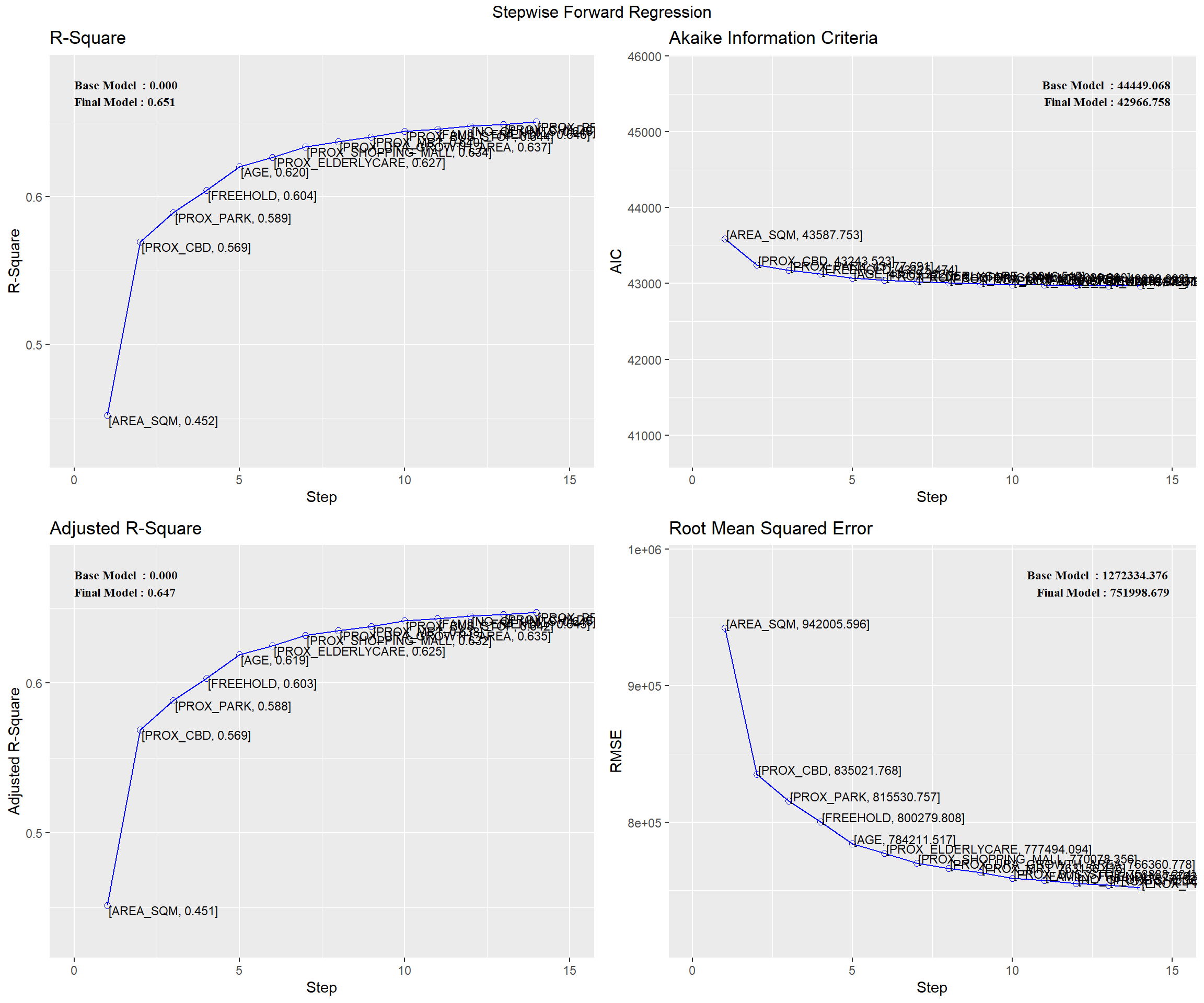
Backward
condo_bw_mlr <- ols_step_backward_p(
  condo_mlr,
  p_val = 0.05,
  details = FALSE
)
condo_bw_mlr
                                     Stepwise Summary
-----------------------------------------------------------------------------------------
Step    Variable                   AIC          SBC         SBIC         R2       Adj. R2
-----------------------------------------------------------------------------------------
 0      Full Model              42970.175    43075.567    38895.493    0.65179    0.64736
 1      PROX_TOP_PRIMARY_SCH    42968.188    43068.310    38893.478    0.65178    0.64761
 2      PROX_SUPERMARKET        42966.534    43061.387    38891.789    0.65170    0.64777
 3      PROX_HAWKER_MARKET      42965.558    43055.141    38890.764    0.65145    0.64777
 4      PROX_KINDERGARTEN       42966.758    43051.072    38891.872    0.65067    0.64723
-----------------------------------------------------------------------------------------

Final Model Output
------------------

                                Model Summary
-----------------------------------------------------------------------------
R                            0.807       RMSE                     751998.679
R-Squared                    0.651       MSE                571471422208.591
Adj. R-Squared               0.647       Coef. Var                    43.168
Pred R-Squared               0.638       AIC                       42966.758
MAE                     414819.628       SBC                       43051.072
-----------------------------------------------------------------------------
 RMSE: Root Mean Square Error
 MSE: Mean Square Error
 MAE: Mean Absolute Error
 AIC: Akaike Information Criteria
 SBC: Schwarz Bayesian Criteria

                                     ANOVA
--------------------------------------------------------------------------------
                    Sum of
                   Squares          DF         Mean Square       F         Sig.
--------------------------------------------------------------------------------
Regression    1.512586e+15          14        1.080418e+14    189.059    0.0000
Residual      8.120609e+14        1421    571471422208.591
Total         2.324647e+15        1435
--------------------------------------------------------------------------------

                                               Parameter Estimates
-----------------------------------------------------------------------------------------------------------------
               model           Beta    Std. Error    Std. Beta       t        Sig           lower          upper
-----------------------------------------------------------------------------------------------------------------
         (Intercept)     527633.222    108183.223                   4.877    0.000     315417.244     739849.200
            AREA_SQM      12777.523       367.479        0.584     34.771    0.000      12056.663      13498.382
                 AGE     -24687.739      2754.845       -0.167     -8.962    0.000     -30091.739     -19283.740
            PROX_CBD     -77131.323      5763.125       -0.263    -13.384    0.000     -88436.469     -65826.176
      PROX_CHILDCARE    -318472.751    107959.512       -0.084     -2.950    0.003    -530249.889    -106695.613
    PROX_ELDERLYCARE     185575.623     39901.864        0.090      4.651    0.000     107302.737     263848.510
PROX_URA_GROWTH_AREA      39163.254     11754.829        0.060      3.332    0.001      16104.571      62221.936
            PROX_MRT    -294745.107     56916.367       -0.112     -5.179    0.000    -406394.234    -183095.980
           PROX_PARK     570504.807     65507.029        0.150      8.709    0.000     442003.938     699005.677
    PROX_PRIMARY_SCH     159856.136     60234.599        0.062      2.654    0.008      41697.849     278014.424
  PROX_SHOPPING_MALL    -220947.251     36561.832       -0.115     -6.043    0.000    -292668.213    -149226.288
       PROX_BUS_STOP     682482.221    134513.243        0.134      5.074    0.000     418616.359     946348.082
         NO_Of_UNITS       -245.480        87.947       -0.053     -2.791    0.005       -418.000        -72.961
     FAMILY_FRIENDLY     146307.576     46893.021        0.057      3.120    0.002      54320.593     238294.560
            FREEHOLD     350599.812     48506.485        0.136      7.228    0.000     255447.802     445751.821
-----------------------------------------------------------------------------------------------------------------plot(condo_bw_mlr)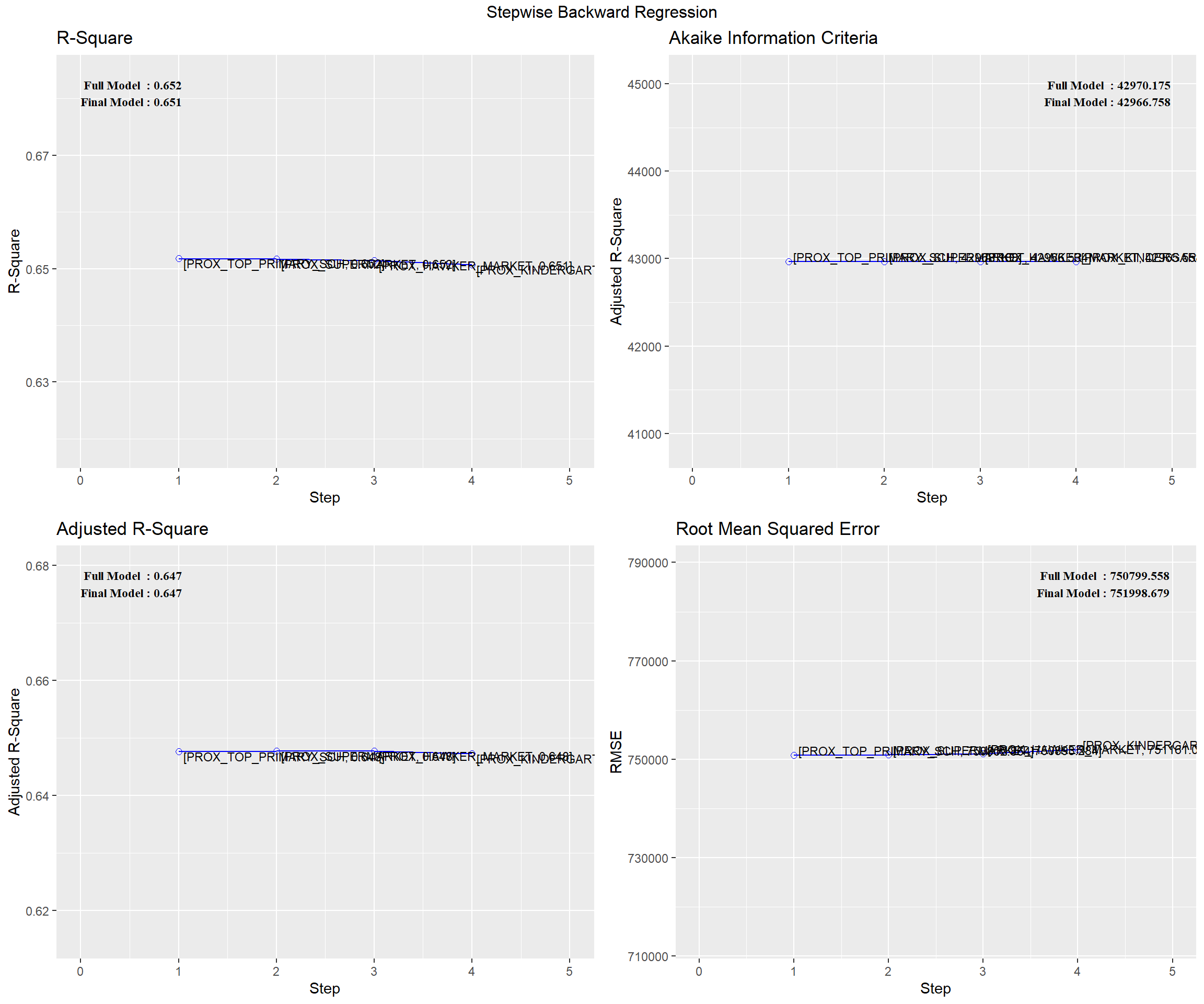
Bi-direction
condo_bi_mlr <- ols_step_both_p(
  condo_mlr,
  p_val = 0.05,
  details = FALSE
)
condo_bi_mlr
                                       Stepwise Summary
---------------------------------------------------------------------------------------------
Step    Variable                       AIC          SBC         SBIC         R2       Adj. R2
---------------------------------------------------------------------------------------------
 0      Base Model                  44449.068    44459.608    40371.745    0.00000    0.00000
 1      AREA_SQM (+)                43587.753    43603.562    39510.883    0.45184    0.45146
 2      PROX_CBD (+)                43243.523    43264.602    39167.182    0.56928    0.56868
 3      PROX_PARK (+)               43177.691    43204.039    39101.331    0.58915    0.58829
 4      FREEHOLD (+)                43125.474    43157.092    39049.179    0.60438    0.60327
 5      AGE (+)                     43069.222    43106.109    38993.167    0.62010    0.61878
 6      PROX_ELDERLYCARE (+)        43046.515    43088.672    38970.548    0.62659    0.62502
 7      PROX_SHOPPING_MALL (+)      43020.990    43068.417    38945.209    0.63367    0.63188
 8      PROX_URA_GROWTH_AREA (+)    43009.092    43061.788    38933.407    0.63720    0.63517
 9      PROX_MRT (+)                42999.058    43057.024    38923.483    0.64023    0.63796
 10     PROX_BUS_STOP (+)           42984.951    43048.186    38909.581    0.64424    0.64175
 11     FAMILY_FRIENDLY (+)         42981.085    43049.590    38905.797    0.64569    0.64296
 12     NO_Of_UNITS (+)             42975.246    43049.021    38900.092    0.64762    0.64465
 13     PROX_CHILDCARE (+)          42971.858    43050.902    38896.812    0.64894    0.64573
 14     PROX_PRIMARY_SCH (+)        42966.758    43051.072    38891.872    0.65067    0.64723
 15     PROX_KINDERGARTEN (+)       42965.558    43055.141    38890.764    0.65145    0.64777
---------------------------------------------------------------------------------------------

Final Model Output
------------------

                                Model Summary
-----------------------------------------------------------------------------
R                            0.807       RMSE                     751161.087
R-Squared                    0.651       MSE                570600646491.086
Adj. R-Squared               0.648       Coef. Var                    43.135
Pred R-Squared               0.638       AIC                       42965.558
MAE                     413583.799       SBC                       43055.141
-----------------------------------------------------------------------------
 RMSE: Root Mean Square Error
 MSE: Mean Square Error
 MAE: Mean Absolute Error
 AIC: Akaike Information Criteria
 SBC: Schwarz Bayesian Criteria

                                     ANOVA
--------------------------------------------------------------------------------
                    Sum of
                   Squares          DF         Mean Square       F         Sig.
--------------------------------------------------------------------------------
Regression    1.514394e+15          15        1.009596e+14    176.936    0.0000
Residual      8.102529e+14        1420    570600646491.086
Total         2.324647e+15        1435
--------------------------------------------------------------------------------

                                               Parameter Estimates
-----------------------------------------------------------------------------------------------------------------
               model           Beta    Std. Error    Std. Beta       t        Sig           lower          upper
-----------------------------------------------------------------------------------------------------------------
         (Intercept)     459826.675    114616.014                   4.012    0.000     234991.777     684661.574
            AREA_SQM      12720.174       368.610        0.581     34.509    0.000      11997.096      13443.252
            PROX_CBD     -75676.065      5816.474       -0.258    -13.011    0.000     -87085.870     -64266.259
           PROX_PARK     575749.528     65523.382        0.151      8.787    0.000     447216.504     704282.552
            FREEHOLD     360203.286     48768.851        0.140      7.386    0.000     264536.552     455870.021
                 AGE     -24697.719      2752.751       -0.167     -8.972    0.000     -30097.615     -19297.824
    PROX_ELDERLYCARE     182435.081     39910.469        0.088      4.571    0.000     104145.268     260724.893
  PROX_SHOPPING_MALL    -224513.955     36588.872       -0.117     -6.136    0.000    -296288.004    -152739.906
PROX_URA_GROWTH_AREA      40145.474     11758.824        0.062      3.414    0.001      17078.942      63212.007
            PROX_MRT    -311753.202     57670.032       -0.119     -5.406    0.000    -424880.814    -198625.590
       PROX_BUS_STOP     711858.014    135420.040        0.140      5.257    0.000     446213.188     977502.840
     FAMILY_FRIENDLY     144034.218     46874.683        0.057      3.073    0.002      52083.153     235985.283
         NO_Of_UNITS       -236.270        88.032       -0.051     -2.684    0.007       -408.956        -63.583
      PROX_CHILDCARE    -336118.857    108331.761       -0.088     -3.103    0.002    -548626.339    -123611.374
    PROX_PRIMARY_SCH     162183.897     60202.895        0.063      2.694    0.007      44087.730     280280.063
   PROX_KINDERGARTEN     141915.768     79726.155        0.029      1.780    0.075     -14477.927     298309.464
-----------------------------------------------------------------------------------------------------------------plot(condo_bi_mlr)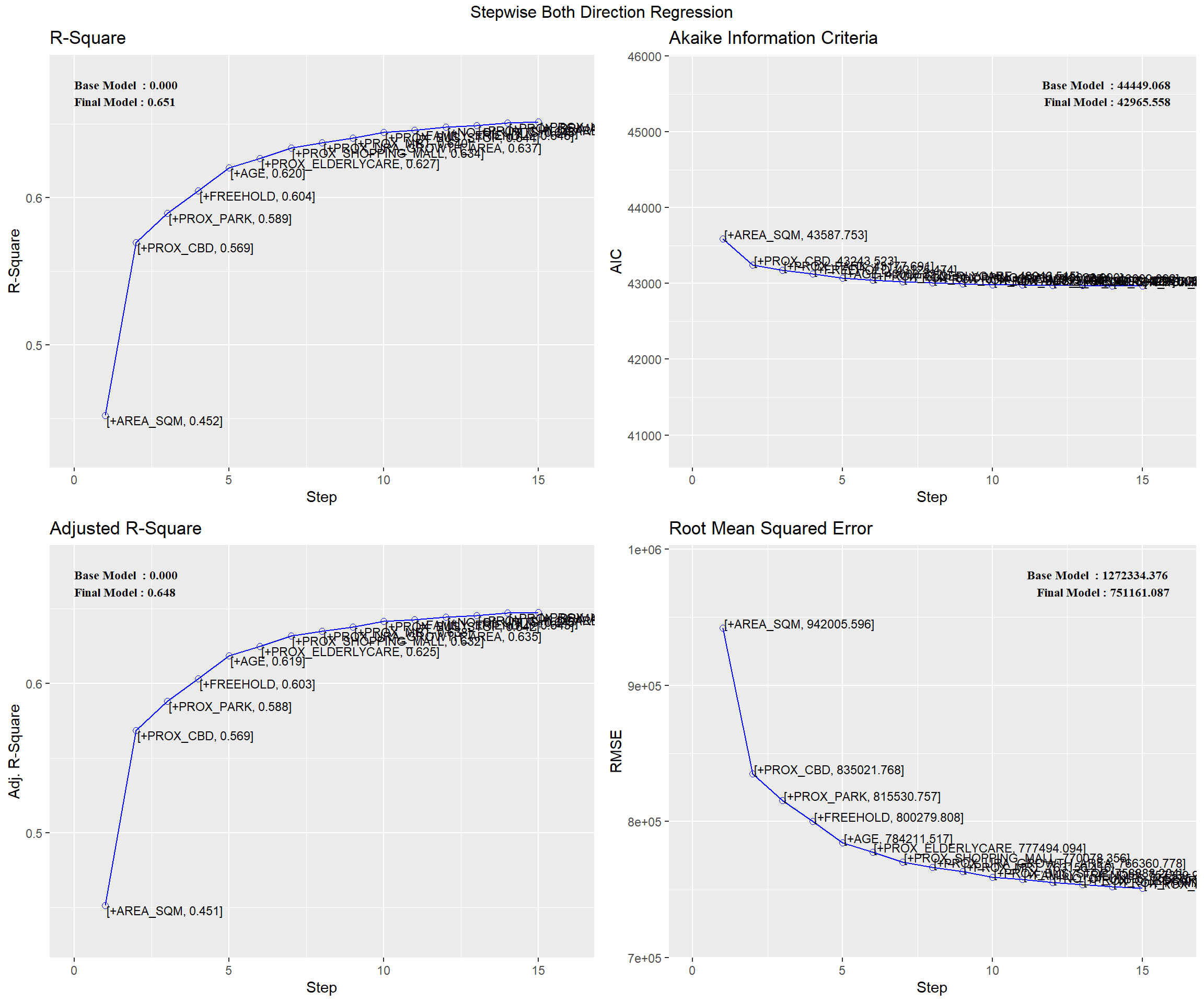
Model Selection
compare_performance() of performance package is used to compare the performance of the models.
metric <- compare_performance(condo_mlr,
                              condo_fw_mlr$model,
                              condo_bw_mlr$model,
                              condo_bi_mlr$model)
gsub() is used to tidy the test value in Name field.
metric$Name <- gsub(".*\\\\([a-zA-Z0-9_]+)\\\\, \\\\model\\\\.*", "\\1", metric$Name)plot(metric)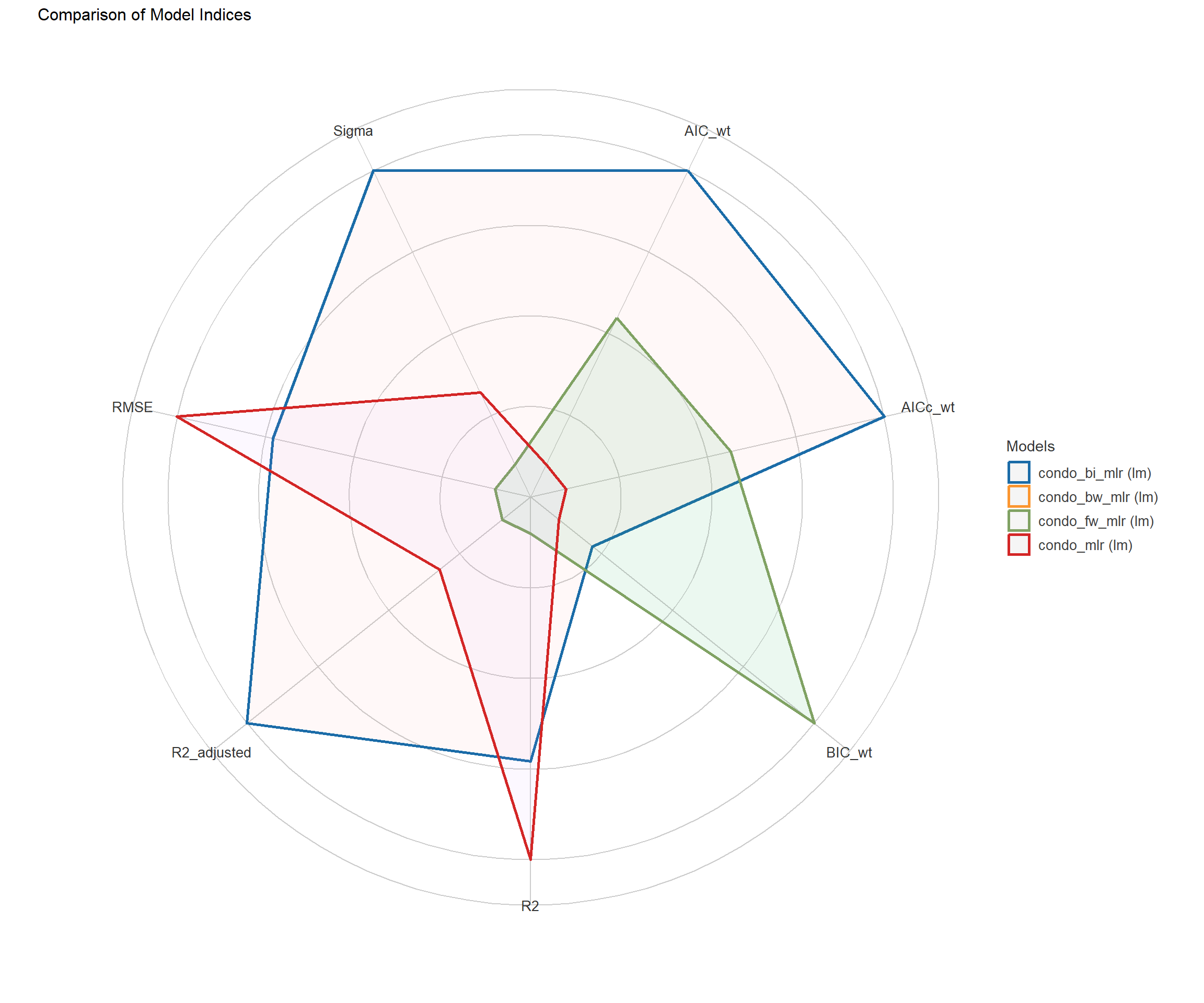
Visualising Model Parameters
ggcoefstats(condo_bi_mlr$model, sort = "ascending")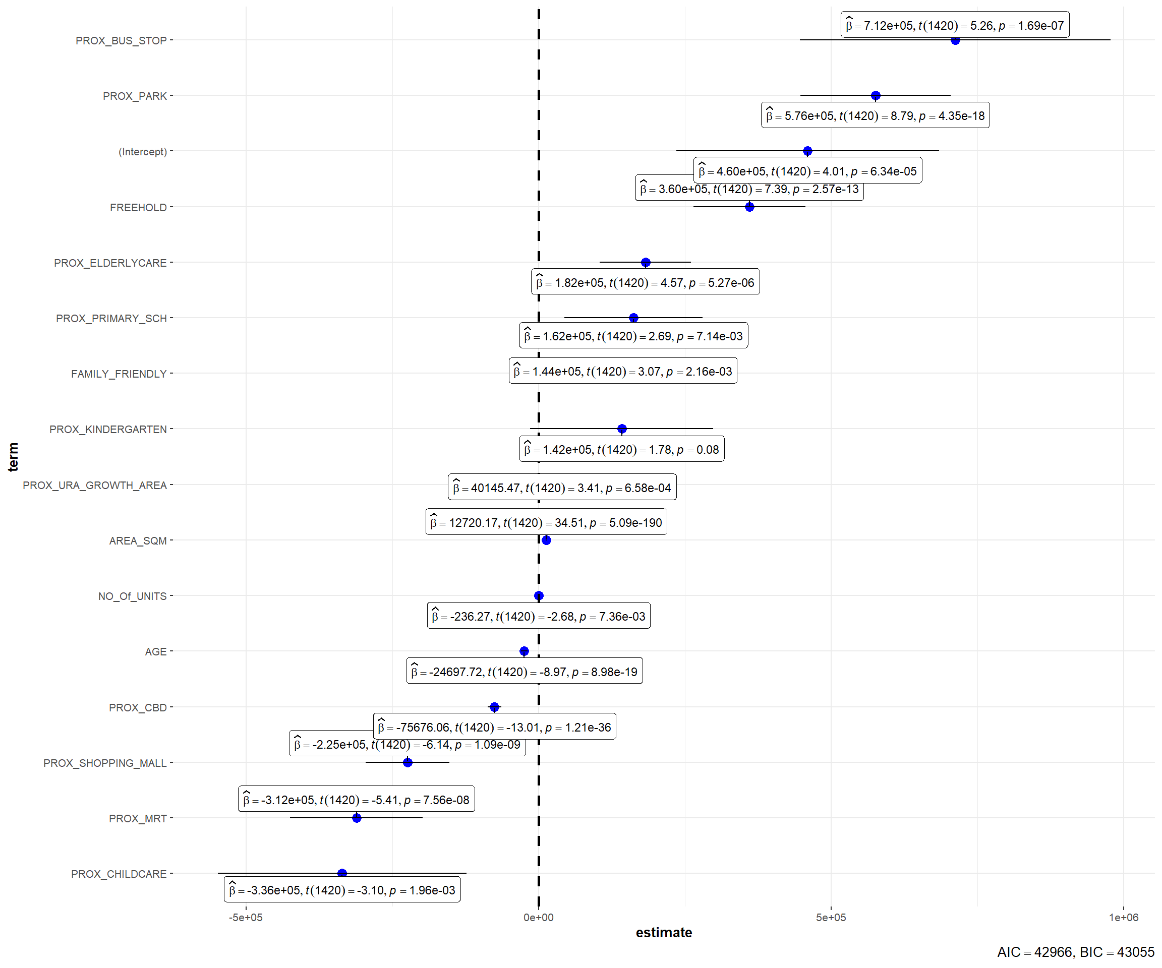
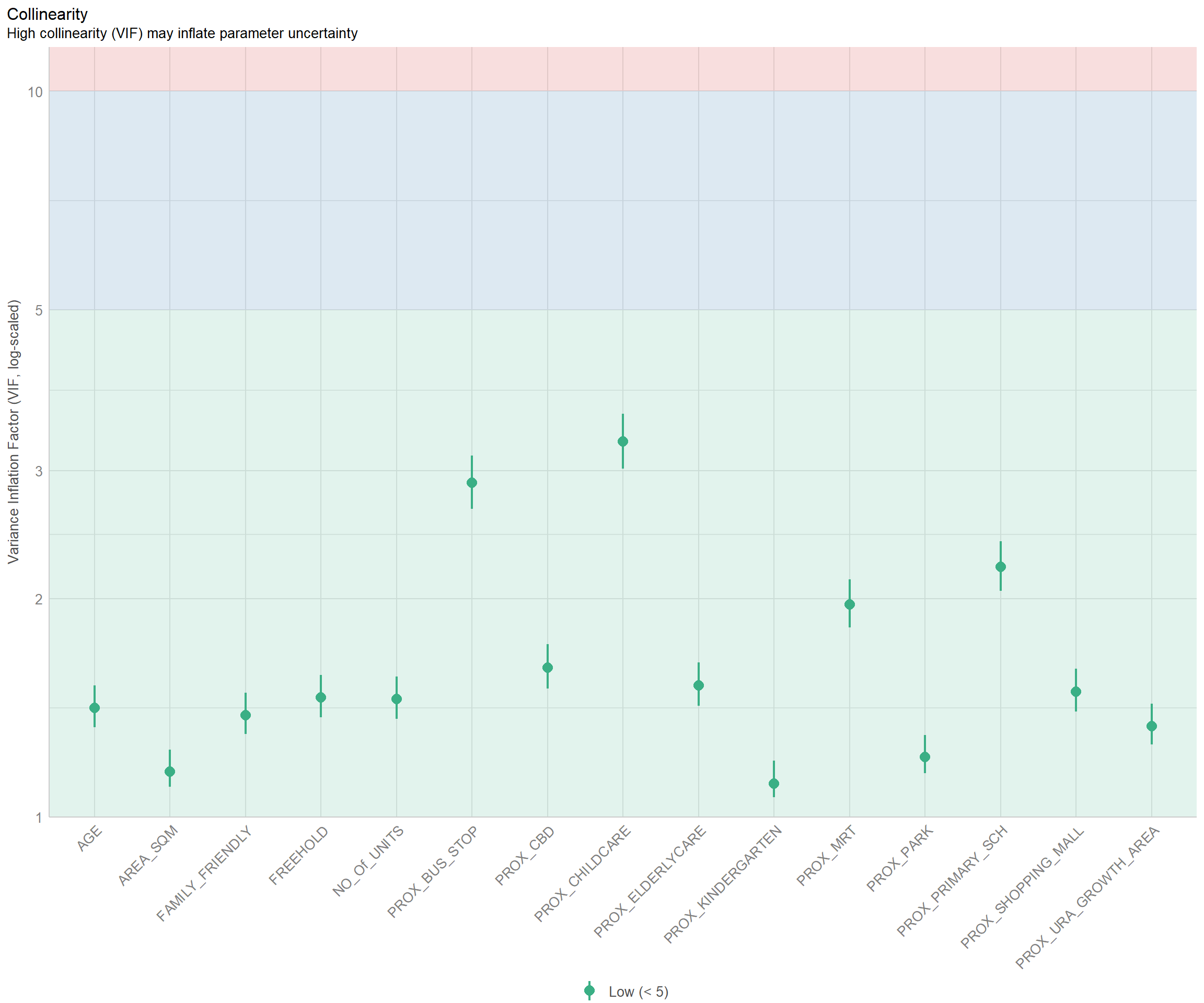
Regression Diagnostics
Checking for multicollinearity
check_collinearity(condo_bi_mlr$model)# Check for Multicollinearity
Low Correlation
Term VIF VIF 95% CI Increased SE Tolerance Tolerance 95% CI
AREA_SQM 1.15 [1.10, 1.24] 1.07 0.87 [0.81, 0.91]
PROX_CBD 1.60 [1.50, 1.73] 1.27 0.62 [0.58, 0.67]
PROX_PARK 1.21 [1.15, 1.30] 1.10 0.83 [0.77, 0.87]
FREEHOLD 1.46 [1.37, 1.57] 1.21 0.68 [0.64, 0.73]
AGE 1.41 [1.33, 1.52] 1.19 0.71 [0.66, 0.75]
PROX_ELDERLYCARE 1.52 [1.42, 1.63] 1.23 0.66 [0.61, 0.70]
PROX_SHOPPING_MALL 1.49 [1.40, 1.60] 1.22 0.67 [0.62, 0.72]
PROX_URA_GROWTH_AREA 1.33 [1.26, 1.43] 1.16 0.75 [0.70, 0.79]
PROX_MRT 1.96 [1.83, 2.13] 1.40 0.51 [0.47, 0.55]
PROX_BUS_STOP 2.89 [2.66, 3.15] 1.70 0.35 [0.32, 0.38]
FAMILY_FRIENDLY 1.38 [1.30, 1.48] 1.18 0.72 [0.67, 0.77]
NO_Of_UNITS 1.45 [1.37, 1.56] 1.21 0.69 [0.64, 0.73]
PROX_CHILDCARE 3.29 [3.02, 3.59] 1.81 0.30 [0.28, 0.33]
PROX_PRIMARY_SCH 2.21 [2.05, 2.40] 1.49 0.45 [0.42, 0.49]
PROX_KINDERGARTEN 1.11 [1.06, 1.20] 1.05 0.90 [0.84, 0.94]plot(check_collinearity(condo_bi_mlr$model)) +
# theme is used to make the display the column name more friendly
theme(axis.text.x = element_text (
angle = 45, hjust = 1
))
Linearity Assumption test
out <- plot(check_model(condo_bi_mlr$model,
                        panel = FALSE))
out[[2]] # have 6 plot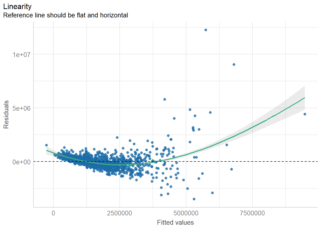
Normality Assumption Test
plot(check_normality(condo_bi_mlr$model))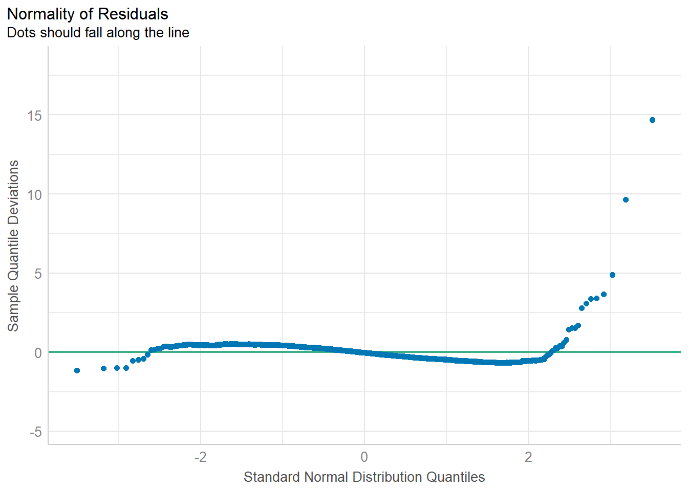
Checking of Outliers
Method => Can be "all" or some of "cook", "pareto", "zscore", "zscore_robust", "iqr", "ci", "eti", "hdi", "bci", "mahalanobis", "mahalanobis_robust", "mcd", "ics", "optics" or "lof".
outliers <- check_outliers(condo_bi_mlr$model,
                           method = "cook")
outliers
OK: No outliers detected.
- Based on the following method and threshold: cook (1).
- For variable: (Whole model)plot(check_outliers(condo_bi_mlr$model,
method = "pareto"))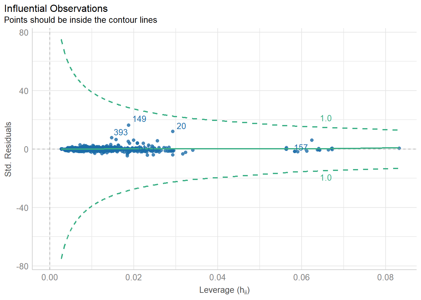
Visualising spatial non-stationary
First, we will export the residual of the hedonic pricing model and save it as a data frame.
mlr_output <- as.data.frame(condo_fw_mlr$model$residuals) %>%
  rename(`FW_MLR_RES` = `condo_fw_mlr$model$residuals`)
Next, we will join the newly created data frame with condo_resale_sf object.
condo_resale_sf <- cbind(condo_resale_sf,
                        mlr_output$FW_MLR_RES) %>%
rename(`MLR_RES` = `mlr_output.FW_MLR_RES`)tmap_mode("plot")
tm_shape(mpsz)+
tmap_options(check.and.fix = TRUE) +
tm_polygons(alpha = 0.4) +
tm_shape(condo_resale_sf) +
tm_dots(col = "MLR_RES",
alpha = 0.6,
style="quantile") 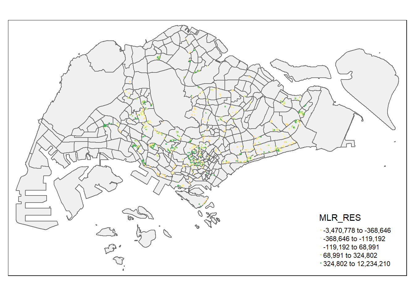
tmap_mode("plot")Spatial Stationary Test
First, we will compute the distance-based weight matrix by using dnearneigh() function of spdep.
condo_resale_sf <- condo_resale_sf %>%
  mutate(nb = st_knn(geometry, k=6,
                     longlat = FALSE),
         wt = st_weights(nb,
                         style = "W"),
         .before = 1)
Next, global_moran_perm() of sfdep is used to perform global Moran permutation test.
global_moran_perm(condo_resale_sf$MLR_RES,
                  condo_resale_sf$nb,
                  condo_resale_sf$wt,
                  alternative = "two.sided",
                  nsim = 99)
    Monte-Carlo simulation of Moran I

data:  x
weights: listw
number of simulations + 1: 100

statistic = 0.32254, observed rank = 100, p-value < 2.2e-16
alternative hypothesis: two.sided