Take-home Exercise 2: Application of Geospatial Analysis Methods to Discover Thailand Drug Abuse at the Province Level

2.1 Exercise Overview

Drug abuse is associated with profound health, financial, and social consequences, making it a critical global issue. Despite numerous efforts to combat the problem, illicit drug use remains highly prevalent, affecting millions of people worldwide. In 2021, it was estimated that 1 in 17 individuals aged 15–64 had used a drug in the past 12 months, with the total number of drug users rising from 240 million in 2011 to 296 million in 2021.

Thailand, in particular, is in a unique geopolitical position near the Golden Triangle of Indochina—the largest drug production site in Asia. This, combined with ongoing transportation infrastructure development, has made Thailand not only a significant market for drug consumption but also a critical transit route for drug trafficking to other countries. As a result, the nation faces a growing challenge in managing the social and health issues associated with drug abuse.

Among Thailand’s youth population, drug abuse is a major social issue. With approximately 2.7 million youths involved in drug use, it is estimated that around 300,000 individuals aged between 15 and 19 require drug treatment. Alarmingly, drug involvement is particularly prevalent among vocational-school students, almost double that of secondary-school students, indicating that certain sub-populations may be at higher risk.

Given this context, the primary objective of this exercise is to explore whether key drug abuse indicators in Thailand are spatially independent or exhibit patterns of spatial dependence. Understanding these spatial dynamics is crucial for identifying clusters, outliers, and potential hotspots that can inform targeted interventions. Additionally, the temporal evolution of these spatial patterns from 2017 to 2022 will be analyzed to uncover trends and shifts over time.

This exercise aims to provide a comprehensive understanding of the spatial and temporal dynamics of drug abuse in Thailand. By identifying areas of concern and tracking their changes over time, the results can support policymakers and stakeholders in designing more effective, location-based strategies to mitigate the impact of drug abuse in the country.

2.2 Data Acquisition

For the purpose of this take-home exercise, two data sets shall be used, they are: Thailand Drug Offenses [2017-2022] at Kaggle. Thailand - Subnational Administrative Boundaries at HDX. You are required to use the province boundary data set.

2.3 Getting Started

For this exercise, the following R packages will be used:

• sf for handling geospatial data.

• spatstat, a comprehensive package for point pattern analysis. We’ll use it to perform first- and second-order spatial point pattern analyses and to derive kernel density estimation (KDE) layers.

• raster, a package for reading, writing, manipulating, and modeling gridded spatial data (rasters). We will use it to convert image outputs generated by spatstat into raster format.

• tmap, a package for creating high-quality static and interactive maps, leveraging the Leaflet API for interactive visualizations.

• tidyverse for performing data science tasks such as importing, wrangling and visualising data.

• RColorBrewer for creating nice looking color palettes especially for thematic maps.

• spdep for spatial dependence analysis, including computing spatial weights and conducting spatial autocorrelation tests such as Moran’s I and Geary’s C

• sfdep for computing spatial weights, global and local spatial autocorrelation statistics

• ggplot2 for data visualization within the tidyverse. It will be used for creating a variety of plots, including temporal line charts and exploratory data visualizations that complement spatial maps

As readr, tidyr and dplyr are part of tidyverse package. The code chunk below will suffice to install and load the required packages in RStudio.

To install and load these packages into the R environment, we use the p_load function from the pacman package:

pacman::p_load(sf, raster, spatstat, tmap, tidyverse, RColorBrewer, spdep, sfdep, ggplot2)

2.4 Importing Data into R

Next, we will import the thai_drug_offenses_2017_2022.csv file into the R environment and save it into an R dataframe called acled_sf. The task can be performed using the read_csv() function from the readr package, as shown below:

thai_drug_offenses <- read.csv("data/archive/thai_drug_offenses_2017_2022.csv")%>% 
  select(-province_th)

drug_summary <- thai_drug_offenses %>%
  group_by(fiscal_year, province_en, types_of_drug_offenses) %>%
  summarize(no_cases = sum(no_cases, na.rm = TRUE), .groups = 'drop')

Notes

We used the select() function to ensure that the province_th column is not included in the dataframe.

We then perform summary operation on the thai_drug_offenses dataset:

• Grouping: The data is grouped by fiscal_year, province_en, and types_of_drug_offenses, which organizes the data by year, province, and type of drug offense.
• Summarizing: For each group, it calculates the total number of cases (no_cases) by summing them while ignoring any missing values (na.rm = TRUE).
• Output: The resulting drug_summary dataset will contain the summarized number of drug offense cases (no_cases) for each combination of year, province, and offense type.

The .groups = 'drop' argument ensures that the grouping is removed from the final summarized data.

We then import the boundaries and provinces of Thailand using the st_read() function to import the tha_adm_rtsd_itos_20210121_shp shapefile into R as a simple feature data frame named regions_sf. We also check the validity of the imported dataset, ensuring that it is in the right format with the st_crs() function:

regions_sf <- st_read(dsn = "data/tha_adm_rtsd_itos_20210121_shp", 
                layer = "tha_admbnda_adm1_rtsd_20220121")

Reading layer `tha_admbnda_adm1_rtsd_20220121' from data source 
  `C:\Users\blzll\OneDrive\Desktop\Y3S1\IS415\Quarto\IS415\Take-home_ex\Take-home_ex02\data\tha_adm_rtsd_itos_20210121_shp' 
  using driver `ESRI Shapefile'
Simple feature collection with 77 features and 16 fields
Geometry type: MULTIPOLYGON
Dimension:     XY
Bounding box:  xmin: 97.34336 ymin: 5.613038 xmax: 105.637 ymax: 20.46507
Geodetic CRS:  WGS 84

st_crs(regions_sf)

Coordinate Reference System:
  User input: WGS 84 
  wkt:
GEOGCRS["WGS 84",
    DATUM["World Geodetic System 1984",
        ELLIPSOID["WGS 84",6378137,298.257223563,
            LENGTHUNIT["metre",1]]],
    PRIMEM["Greenwich",0,
        ANGLEUNIT["degree",0.0174532925199433]],
    CS[ellipsoidal,2],
        AXIS["latitude",north,
            ORDER[1],
            ANGLEUNIT["degree",0.0174532925199433]],
        AXIS["longitude",east,
            ORDER[2],
            ANGLEUNIT["degree",0.0174532925199433]],
    ID["EPSG",4326]]

2.5 Data Wrangling

Before proceed we will do some data wrangling, this step primarily consist of checking for possible mismatches due to differences in the imported datasets. We will create a function to identify this.

# Function to check province differences
prov_diff <- function(thai_drug_offenses_provinces, regions_sf_provinces) {
  # Create sets for efficient comparison
  drug_set <- unique(thai_drug_offenses_provinces)
  regions_set <- unique(regions_sf_provinces)
  
  # Check for mismatches
  missing_in_regions <- setdiff(drug_set, regions_set)
  missing_in_drug <- setdiff(regions_set, drug_set)
  
  if (length(missing_in_regions) == 0 && length(missing_in_drug) == 0) {
    cat("All province names match.\n")
  } else {
    cat("There are mismatches in province names.\n")
    if (length(missing_in_regions) > 0) {
      cat("Missing in regions_sf:", paste(missing_in_regions, collapse = ", "), "\n")
    }
    if (length(missing_in_drug) > 0) {
      cat("Missing in drug_sf:", paste(missing_in_drug, collapse = ", "), "\n")
    }
  }
}

prov_diff(unique(thai_drug_offenses$province_en), unique(regions_sf$ADM1_EN))

There are mismatches in province names.
Missing in regions_sf: Loburi, buogkan 
Missing in drug_sf: Lop Buri, Bueng Kan 

Based on the derived results, we would need to reassign the misaligned values such that they match exactly. In the code chunk below, we will perform the reassignment in the regions_sf

thai_drug_offenses <- thai_drug_offenses %>%
  mutate(province_en = case_when(
    province_en == "Loburi" ~ "Lop Buri",
    province_en == "buogkan" ~ "Bueng Kan",
    TRUE ~ province_en
  ))

prov_diff(unique(thai_drug_offenses$province_en), unique(regions_sf$ADM1_EN))

All province names match.

We will then join both datasets togther based on the province_en and ADM1_EN columns

drug_region_1 <- left_join(thai_drug_offenses, regions_sf, by = c("province_en" = "ADM1_EN")) %>%
  select(1:6, "date", "geometry")

We then perform data validation checks on the newly created drug_region_1 dataset, checking for missing values in key columns: geometry, province_en, types_of_drug_offenses, and no_cases. It uses the summarise() function to count how many NA values exist in each of these columns, helping to identify any incomplete or missing data.

# Check for null values in key columns
na_count <- drug_region_1 %>%
  summarise(na_geometry = sum(is.na(geometry)),
            na_province = sum(is.na(province_en)),
            na_drug_offense = sum(is.na(types_of_drug_offenses)),
            na_cases = sum(is.na(no_cases)))

print(na_count)

  na_geometry na_province na_drug_offense na_cases
1           0           0               0        0

We then look for duplicate rows by grouping the data by province_en, fiscal_year, and types_of_drug_offenses. If any rows have the same combination of these fields (i.e., they are duplicates), they will be filtered and displayed; otherwise, a message indicating no duplicates will be printed. These steps ensure data quality before proceeding with any spatial or statistical analysis.

duplicates <- drug_region_1 %>%
  group_by(province_en, fiscal_year, types_of_drug_offenses) %>%
  filter(n() > 1) %>%
  ungroup()

if (nrow(duplicates) > 0) {
  cat("Duplicates found:\n")
  print(duplicates)
} else {
  cat("No duplicates found.\n")
}

No duplicates found.

We then ensure that drug_region_1 is an sf object by using the st_crs() function, which returns the coordinate reference system (CRS) if the object is spatial, converting the drug_region_1 data frame into an sf object using st_as_sf(), specifying EPSG:4326 as the CRS. This corresponds to the WGS 84 geographic coordinate system which is suitable for country of Thailand. This conversion is necessary to perform spatial analysis, as it ensures the dataset includes spatial information with proper geographic coordinates.

# check if drug_region_1 is an sf object
st_crs(drug_region_1)

Coordinate Reference System: NA

# Convert data frame to sf object and specify the CRS (EPSG:4326)
drug_region_thailand_sf <- st_as_sf(drug_region_1, crs = 4326)

write_rds(drug_region_thailand_sf, "data/rds/drug_region_thailand_sf.rds")
drug_region_thailand_sf <- read_rds("data/rds/drug_region_thailand_sf.rds")

2.6 Global Measures of Spatial Autocorrelation

Global measures of spatial autocorrelation, such as Moran’s I and Geary’s C, are critical in understanding the overall spatial structure of geographic data. They help detect patterns of clustering or dispersion by assessing whether similar values occur near each other across an entire study area. This insight is essential for identifying spatial dependencies and guiding decisions in fields like epidemiology, economics, and environmental science. By quantifying spatial relationships on a broad scale, global measures provide a foundational perspective for spatial analysis.

num_colors <- length(unique(regions_sf$ADM1_EN))
colors <- brewer.pal(n = num_colors, name = "Set1")

# as there are 77 provinces in thailand
tmap_options(max.categories = 77)

tm_shape(regions_sf) +
  tm_polygons(col = "ADM1_EN", palette = colors) +
  tm_layout(main.title = "Provinces in Thailand",
            main.title.position = "center",
            main.title.size = 1.6,
            legend.outside = TRUE) +
  tm_legend(title = "Provinces")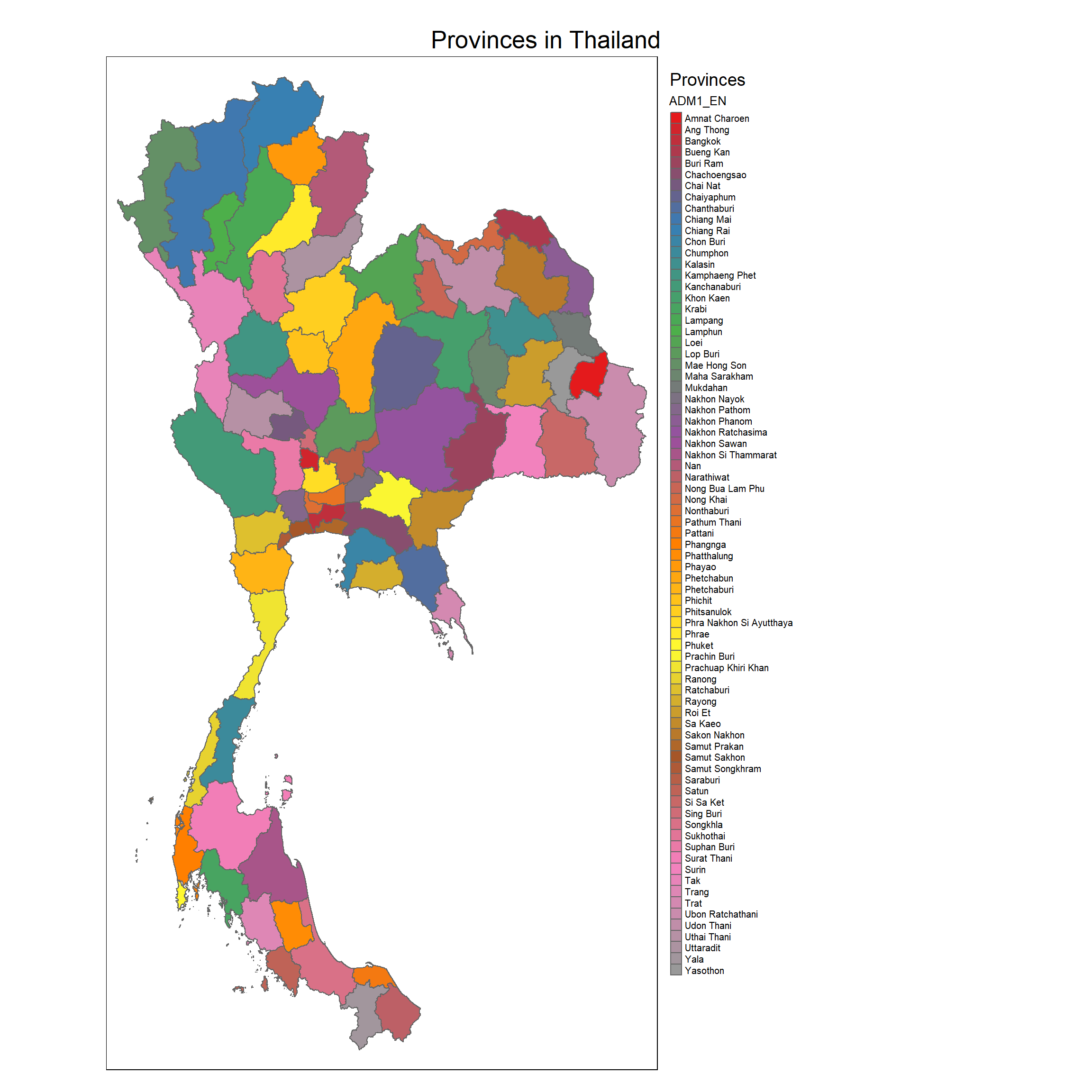

2.6.1 Defining Scope of Analysis

To ensure a data-driven analysis of drug-related offenses, we aim to focus exclusively on cases that have resulted in concrete legal outcomes, such as convictions or possession cases. cases based solely on suspicion may not lead to prosecution or final legal action, potentially inflating the data without accurately reflecting the true extent of confirmed criminal activity. By narrowing our scope to finalized or substantiated cases, we intend to provide more reliable insights into the patterns of drug-related crime and its impact.

# Group by types_of_drug_offenses and summarize by summing the no_cases
top_drug_offenses <- thai_drug_offenses %>%
  filter(!grepl("suspect", types_of_drug_offenses, ignore.case = TRUE)) %>%
  group_by(types_of_drug_offenses) %>%
  summarise(total_cases = sum(no_cases, na.rm = TRUE)) %>%
  arrange(desc(total_cases))

# View non-suspicion based types of drug offenses
top_drug_offenses

# A tibble: 8 × 2
  types_of_drug_offenses                     total_cases
  <chr>                                            <int>
1 drug_use_cases                                  915529
2 possession_cases                                538893
3 possession_with_intent_to_distribute_cases      341283
4 trafficking_cases                                68379
5 production_cases                                 56892
6 conspiracy_cases                                   920
7 import_cases                                       860
8 export_cases                                        84

We are further refining our analysis exclusively on drug use cases. This choice is driven by the nature of these offenses, which represent direct instances of illicit drug consumption and are critical to understanding the broader context of drug-related issues in Thailand. Unlike cases that involve suspicion or potential possession, drug use cases have clear legal implications and societal impacts, making them essential for our analysis. By focusing solely on these confirmed instances, we aim to provide accurate insights into the patterns of drug use and its repercussions.

drug_region_thailand_sf <- drug_region_thailand_sf %>% filter(types_of_drug_offenses == "drug_use_cases")

Focusing exclusively on drug use cases allows us to concentrate our efforts on a significant area of concern, thereby providing clearer recommendations for law enforcement and policy development. This targeted approach ensures that our insights align with the most impactful drug-related offenses, facilitating more effective interventions and resource allocation.

region_2017_sf <- drug_region_thailand_sf %>% filter(fiscal_year == 2017)
region_2018_sf <- drug_region_thailand_sf %>% filter(fiscal_year == 2018)
region_2019_sf <- drug_region_thailand_sf %>% filter(fiscal_year == 2019)
region_2020_sf <- drug_region_thailand_sf %>% filter(fiscal_year == 2020)
region_2021_sf <- drug_region_thailand_sf %>% filter(fiscal_year == 2021)
region_2022_sf <- drug_region_thailand_sf %>% filter(fiscal_year == 2022)

2.6.2 Computing Contiguity Neighbours

Year 2017

thailand_nb_q <- st_contiguity(region_2017_sf, queen=TRUE)
summary(thailand_nb_q)

Neighbour list object:
Number of regions: 77 
Number of nonzero links: 352 
Percentage nonzero weights: 5.93692 
Average number of links: 4.571429 
1 region with no links:
68
2 disjoint connected subgraphs
Link number distribution:

 0  1  2  3  4  5  6  7  8  9 
 1  1  5 17 15 17 10  5  4  2 
1 least connected region:
14 with 1 link
2 most connected regions:
28 48 with 9 links

1 region with no links can be observed in the summary above. This is due to the island province of Phuket having no direct land neighbours, and being connected to Phangnga province via a bridge. As such, we can manually assign Phuket a neighbor, Phangnga, to help avoid issues in the spatial analysis, particularly with Moran’s I, which requires each region to have at least one neighbor.

The following code chunk finds the index positions of the provinces “Phuket” and “Phangnga” within the region_2017_sf spatial data frame.

phuket_index <- which(region_2017_sf$province_en == "Phuket")
phangnga_index <- which(region_2017_sf$province_en == "Phangnga")

Purpose: This code modifies the neighborhood relationship between “Phuket” and “Phangnga” by manually assigning them as neighbors to each other within the thailand_nb_q object.

thailand_nb_q[phuket_index][1] <- phangnga_index
thailand_nb_q[phangnga_index][2] <- phuket_index

As seen from the summary above all regions are linked and have at least 1 neighbour

Computing Row-Standardised Weight Matrix

Next, we need to assign spatial weights to each neighboring polygon.

st_weights() function from sfdep packge can be used to supplement a neighbour list with spatial weights based on the chosen coding scheme. There are as least 5 different coding scheme styles supported by this function:

• B is the basic binary coding

• W is row standardised (sums over all links to n)

• C is globally standardised (sums over all links to n)

• U is equal to C divided by the number of neighbours (sums over all links to unity)

• S is the variance-stabilizing coding scheme proposed by Tiefelsdorf et al. (1999) (sums over all links to n).

In this study, we will use row-standardised weight matrix (style="W"). Row standardisation of a matrix ensure that the sum of the values across each row add up to 1. This is accomplished by assigning the fraction 1/(# of neighbors) to each neighboring county then summing the weighted income values. Row standardisation ensures that all weights are between 0 and 1. This facilities the interpretation of operation with the weights matrix as an averaging of neighboring values, and allows for the spatial parameter used in our analyses to be comparable between models.

thailand_wm_rs <- st_weights(thailand_nb_q, style = "W")

We will mutate the newly created neighbour list object thailand_nb_q and weight matrix thailand_wm_rs into our existing region_2017_sf. The result will be a new object, which we will call wm_q_<current-year>.

wm_q_2017 <- region_2017_sf %>%
  mutate(nb = thailand_nb_q,
         wt = thailand_wm_rs,
         .before = 1) 

Global Moran’s I

Global Moran’s I

moranI <- global_moran(wm_q_2017$no_cases,
                        wm_q_2017$nb,
                        wm_q_2017$wt)
moranI

$I
[1] 0.08216344

$K
[1] 30.4821

Global Moran’s I test

global_moran_test_2017 <- global_moran_test(wm_q_2017$no_cases,
                            wm_q_2017$nb,
                            wm_q_2017$wt,
                            alternative = "greater")
global_moran_test_2017_statistics <- global_moran_test_2017$estimate["Moran I statistic"]
global_moran_test_2017_p_value <- global_moran_test_2017$p.value
global_moran_test_2017

    Moran I test under randomisation

data:  x  
weights: listw    

Moran I statistic standard deviate = 1.5745, p-value = 0.05768
alternative hypothesis: greater
sample estimates:
Moran I statistic       Expectation          Variance 
      0.082163436      -0.013157895       0.003665038 

For the year of 2017, the Moran I statistic shows slight positive spatial autocorrelation, meaning there is some clustering of similar values of drug-related cases, but this clustering is weak and not statistically significant at the 5% level (though close, with a p-value of 0.0577). There is weak evidence suggesting that nearby provinces might have similar levels of drug-related cases, but the relationship is not strong enough to definitively conclude spatial clustering. As such, further investigation is needed to show stronger spatial autocorrelation.

Global Moran’s I permutation test

set.seed(4242)
gmoranMC_2017 <- global_moran_perm(wm_q_2017$no_cases,
                  wm_q_2017$nb,
                  wm_q_2017$wt,
                  nsim = 999)
gmoranMC_2017

    Monte-Carlo simulation of Moran I

data:  x 
weights: listw  
number of simulations + 1: 1000 

statistic = 0.082163, observed rank = 933, p-value = 0.134
alternative hypothesis: two.sided

Global Geary’s C

Introduced by Geary, Geary’s C statistic studies the degree of intensity of a given feature in spatial objects described with the use of a weight matrix. Similarly to Moran’s analysis, Geary’s C can be used to quantify the extent of spatial autocorrelation in the data.

Global Geary’s C test

The Global Geary’s C test, which can be implemented using the global_c_test() function from the sfdep package.

global_c_test_2017 <- global_c_test(wm_q_2017$no_cases,
                                    wm_q_2017$nb,
                                    wm_q_2017$wt,
                                    alternative = "greater")
global_c_test_2017_statistics <- global_c_test_2017$estimate ["Geary C statistic"]
global_c_test_2017_p_value <- global_c_test_2017$p.value
global_c_test_2017

    Geary C test under randomisation

data:  x 
weights: listw   

Geary C statistic standard deviate = -0.17983, p-value = 0.5714
alternative hypothesis: Expectation greater than statistic
sample estimates:
Geary C statistic       Expectation          Variance 
       1.02584500        1.00000000        0.02065461 

Global Geary’s C Permutation Test

Similar to what we did in Moran’s I test, we will use global_c_perm() function from sfdep package with nsim = 999 which represent 1000 Monte Carlo simulations to be carried out.

set.seed(4242)
bperm_2017 <- global_c_perm(wm_q_2017$no_cases,
                  wm_q_2017$nb,
                  wm_q_2017$wt,
                  nsim = 999)
bperm_2017

    Monte-Carlo simulation of Geary C

data:  x 
weights: listw  
number of simulations + 1: 1000 

statistic = 1.0258, observed rank = 565, p-value = 0.565
alternative hypothesis: greater

Year 2018

Similar that of 2017, we will compute a contiguity weight matrix for the study area, assigning spatial weights to each neighboring polygon, while also manually assigning “Phuket” and “Phangnga” as neighbours.

thailand_nb_q <- st_contiguity(region_2018_sf, queen=TRUE)

The following code chunk finds the index positions of the provinces “Phuket” and “Phangnga” within the region_2017_sf spatial data frame, assigning them as neighbors to each other within the thailand_nb_q object.

phuket_index <- which(region_2018_sf$province_en == "Phuket")
phangnga_index <- which(region_2018_sf$province_en == "Phangnga")

thailand_nb_q[phuket_index][1] <- phangnga_index
thailand_nb_q[phangnga_index][2] <- phuket_index

Computing Row-Standardised Weight Matrix

Using the contiguity weight matrix, we will use row-standardised weight matrix (style = “W”).

thailand_wm_rs <- st_weights(thailand_nb_q, style = "W")

We then mutate the newly created neighbour list object thailand_nb_q and weight matrix thailand_wm_rs into our existing region_2018_sf. The result will be a new object, which we will call wm_q_<current-year>.

wm_q_2018 <- region_2018_sf %>%
  mutate(nb = thailand_nb_q,
         wt = thailand_wm_rs,
         .before = 1) 

Global Moran’s I

Global Moran’s I

moranI <- global_moran(wm_q_2018$no_cases,
                        wm_q_2018$nb,
                        wm_q_2018$wt)
moranI

$I
[1] 0.09520252

$K
[1] 27.02001

Global Moran’s I test

global_moran_test_2018 <- global_moran_test(wm_q_2018$no_cases,
                            wm_q_2018$nb,
                            wm_q_2018$wt,
                            alternative = "greater")
global_moran_test_2018_statistics <- global_moran_test_2018$estimate["Moran I statistic"]
global_moran_test_2018_p_value <- global_moran_test_2018$p.value
global_moran_test_2018

    Moran I test under randomisation

data:  x  
weights: listw    

Moran I statistic standard deviate = 1.7246, p-value = 0.0423
alternative hypothesis: greater
sample estimates:
Moran I statistic       Expectation          Variance 
      0.095202524      -0.013157895       0.003947668 

In 2018, the results of the Moran’s I test reveal a slight positive spatial autocorrelation for drug-related cases in Thailand, indicated by a Moran I statistic of 0.0952. This suggests that there is some degree of clustering among provinces with similar levels of drug-related incidents. However, the significance of this clustering is marginal, as evidenced by the p-value of 0.0423, which is just below the conventional threshold of 0.05 for statistical significance.

While the results imply a weak tendency for nearby provinces to exhibit similar drug-related case counts, the evidence is insufficient to draw definitive conclusions about robust spatial clustering. The expectation value of -0.0132 and variance of 0.0039 further support the interpretation that, although there are clusters present, they do not exhibit a strong or clear pattern. This indicates a need for additional analyses or data to better understand the underlying dynamics of drug use in the region. Authorities may consider more detailed investigations to explore factors influencing these patterns, such as socio-economic conditions, access to treatment, or enforcement measures in surrounding areas.

Global Moran’s I permutation test

set.seed(4242)
gmoranMC_2018 <- global_moran_perm(wm_q_2018$no_cases,
                  wm_q_2018$nb,
                  wm_q_2018$wt,
                  nsim = 999)
gmoranMC_2018

    Monte-Carlo simulation of Moran I

data:  x 
weights: listw  
number of simulations + 1: 1000 

statistic = 0.095203, observed rank = 943, p-value = 0.114
alternative hypothesis: two.sided

Global Geary’s C

Introduced by Geary, Geary’s C statistic studies the degree of intensity of a given feature in spatial objects described with the use of a weight matrix. Similarly to Moran’s analysis, Geary’s C can be used to quantify the extent of spatial autocorrelation in the data.

Global Geary’s C test

The Global Geary’s C test, which can be implemented using the global_c_test() function from the sfdep package.

global_c_test_2018 <- global_c_test(wm_q_2018$no_cases,
                                    wm_q_2018$nb,
                                    wm_q_2018$wt,
                                    alternative = "greater")
global_c_test_2018_statistics <- global_c_test_2018$estimate ["Geary C statistic"]
global_c_test_2018_p_value <- global_c_test_2018$p.value
global_c_test_2018

    Geary C test under randomisation

data:  x 
weights: listw   

Geary C statistic standard deviate = -0.026547, p-value = 0.5106
alternative hypothesis: Expectation greater than statistic
sample estimates:
Geary C statistic       Expectation          Variance 
       1.00365196        1.00000000        0.01892375 

Global Geary’s C Permutation Test

Similar to what we did in Moran’s I test, we will use global_c_perm() function from sfdep package with nsim = 999 which represent 1000 Monte Carlo simulations to be carried out.

set.seed(4242)
bperm_2018 <- global_c_perm(wm_q_2018$no_cases,
                  wm_q_2018$nb,
                  wm_q_2018$wt,
                  nsim = 999)
bperm_2018

    Monte-Carlo simulation of Geary C

data:  x 
weights: listw  
number of simulations + 1: 1000 

statistic = 1.0037, observed rank = 524, p-value = 0.524
alternative hypothesis: greater

Year 2019

Similar that of the previous years, we will compute a contiguity weight matrix for the study area, assigning spatial weights to each neighboring polygon, while also manually assigning “Phuket” and “Phangnga” as neighbours.

thailand_nb_q <- st_contiguity(region_2019_sf, queen=TRUE)

The following code chunk finds the index positions of the provinces “Phuket” and “Phangnga” within the region_2017_sf spatial data frame, assigning them as neighbors to each other within the thailand_nb_q object.

phuket_index <- which(region_2019_sf$province_en == "Phuket")
phangnga_index <- which(region_2019_sf$province_en == "Phangnga")

thailand_nb_q[phuket_index][1] <- phangnga_index
thailand_nb_q[phangnga_index][2] <- phuket_index

Computing Row-Standardised Weight Matrix

Using the contiguity weight matrix, we will use row-standardised weight matrix (style = “W”).

thailand_wm_rs <- st_weights(thailand_nb_q, style = "W")

We then mutate the newly created neighbour list object thailand_nb_q and weight matrix thailand_wm_rs into our existing region_2018_sf. The result will be a new object, which we will call wm_q_<current-year>.

wm_q_2019 <- region_2019_sf %>%
  mutate(nb = thailand_nb_q,
         wt = thailand_wm_rs,
         .before = 1) 

Global Moran’s I

Global Moran’s I

moranI <- global_moran(wm_q_2019$no_cases,
                        wm_q_2019$nb,
                        wm_q_2019$wt)
moranI

$I
[1] 0.1410203

$K
[1] 13.70039

Global Moran’s I test

global_moran_test_2019 <- global_moran_test(wm_q_2019$no_cases,
                            wm_q_2019$nb,
                            wm_q_2019$wt,
                            alternative = "greater")
global_moran_test_2019_statistics <- global_moran_test_2019$estimate["Moran I statistic"]
global_moran_test_2019_p_value <- global_moran_test_2019$p.value
global_moran_test_2019

    Moran I test under randomisation

data:  x  
weights: listw    

Moran I statistic standard deviate = 2.1728, p-value = 0.0149
alternative hypothesis: greater
sample estimates:
Moran I statistic       Expectation          Variance 
      0.141020279      -0.013157895       0.005035023 

In 2019, the results of the Moran’s I test indicate a moderate positive spatial autocorrelation for drug-related cases in Thailand, reflected by a Moran I statistic of 0.1410. This suggests a more pronounced clustering effect, where nearby provinces are likely to have similar levels of drug-related incidents.

The p-value of 0.0149 is statistically significant, indicating that the observed clustering is unlikely to be due to random chance at the 5% significance level. This finding reinforces the notion that there are regions in Thailand where drug-related cases are concentrated, pointing to potential hotspots that may require targeted interventions.

Global Moran’s I permutation test

set.seed(4242)
gmoranMC_2019 <- global_moran_perm(wm_q_2019$no_cases,
                  wm_q_2019$nb,
                  wm_q_2019$wt,
                  nsim = 999)
gmoranMC_2019

    Monte-Carlo simulation of Moran I

data:  x 
weights: listw  
number of simulations + 1: 1000 

statistic = 0.14102, observed rank = 975, p-value = 0.05
alternative hypothesis: two.sided

Global Geary’s C

Introduced by Geary, Geary’s C statistic studies the degree of intensity of a given feature in spatial objects described with the use of a weight matrix. Similarly to Moran’s analysis, Geary’s C can be used to quantify the extent of spatial autocorrelation in the data.

Global Geary’s C test

The Global Geary’s C test, which can be implemented using the global_c_test() function from the sfdep package.

global_c_test_2019 <- global_c_test(wm_q_2019$no_cases,
                                    wm_q_2019$nb,
                                    wm_q_2019$wt,
                                    alternative = "greater")
global_c_test_2019_statistics <- global_c_test_2019$estimate ["Geary C statistic"]
global_c_test_2019_p_value <- global_c_test_2019$p.value
global_c_test_2019

    Geary C test under randomisation

data:  x 
weights: listw   

Geary C statistic standard deviate = 0.7522, p-value = 0.226
alternative hypothesis: Expectation greater than statistic
sample estimates:
Geary C statistic       Expectation          Variance 
       0.91669667        1.00000000        0.01226465 

Global Geary’s C Permutation Test

Similar to what we did in Moran’s I test, we will use global_c_perm() function from sfdep package with nsim = 999 which represent 1000 Monte Carlo simulations to be carried out.

set.seed(4242)
bperm_2019 <- global_c_perm(wm_q_2019$no_cases,
                  wm_q_2019$nb,
                  wm_q_2019$wt,
                  nsim = 999)
bperm_2019

    Monte-Carlo simulation of Geary C

data:  x 
weights: listw  
number of simulations + 1: 1000 

statistic = 0.9167, observed rank = 204, p-value = 0.204
alternative hypothesis: greater

Year 2020

Similar that of the previous years, we will compute a contiguity weight matrix for the study area, assigning spatial weights to each neighboring polygon, while also manually assigning “Phuket” and “Phangnga” as neighbours.

thailand_nb_q <- st_contiguity(region_2020_sf, queen=TRUE)

The following code chunk finds the index positions of the provinces “Phuket” and “Phangnga” within the region_2017_sf spatial data frame, assigning them as neighbors to each other within the thailand_nb_q object.

phuket_index <- which(region_2020_sf$province_en == "Phuket")
phangnga_index <- which(region_2020_sf$province_en == "Phangnga")

thailand_nb_q[phuket_index][1] <- phangnga_index
thailand_nb_q[phangnga_index][2] <- phuket_index

Computing Row-Standardised Weight Matrix

Using the contiguity weight matrix, we will use row-standardised weight matrix (style = “W”).

thailand_wm_rs <- st_weights(thailand_nb_q, style = "W")

We then mutate the newly created neighbour list object thailand_nb_q and weight matrix thailand_wm_rs into our existing region_2018_sf. The result will be a new object, which we will call wm_q_<current-year>.

wm_q_2020 <- region_2020_sf %>%
  mutate(nb = thailand_nb_q,
         wt = thailand_wm_rs,
         .before = 1) 

Global Moran’s I

Global Moran’s I

moranI <- global_moran(wm_q_2020$no_cases,
                        wm_q_2020$nb,
                        wm_q_2020$wt)
moranI

$I
[1] 0.0874654

$K
[1] 10.43646

Global Moran’s I test

global_moran_test_2020 <- global_moran_test(wm_q_2020$no_cases,
                            wm_q_2020$nb,
                            wm_q_2020$wt,
                            alternative = "greater")
global_moran_test_2020_statistics <- global_moran_test_2020$estimate["Moran I statistic"]
global_moran_test_2020_p_value <- global_moran_test_2020$p.value
global_moran_test_2020

    Moran I test under randomisation

data:  x  
weights: listw    

Moran I statistic standard deviate = 1.382, p-value = 0.08349
alternative hypothesis: greater
sample estimates:
Moran I statistic       Expectation          Variance 
      0.087465400      -0.013157895       0.005301475 

For the year 2020, the results of the Moran’s I test reveal a slight positive spatial autocorrelation for drug-related cases in Thailand, with a Moran I statistic of 0.0875. This indicates that there is some level of clustering of similar values, although the strength of this clustering is weak.

The p-value of 0.08349 suggests that the observed spatial autocorrelation is not statistically significant at the conventional 5% level, indicating that the clustering might be due to random chance rather than a definitive spatial pattern. Despite being close to significance, this p-value reflects uncertainty regarding the presence of meaningful spatial clusters.

With an expectation value of -0.0132 and a variance of 0.0053, the results imply that while there is a slight tendency for neighboring provinces to exhibit similar drug-related cases, the evidence is insufficient to draw strong conclusions about spatial clustering. Authorities may need to continue monitoring drug-related incidents in this year, as the potential for clustering exists, but further analysis and data may be required to identify any significant patterns or trends.

Global Moran’s I permutation test

set.seed(4242)
gmoranMC_2020 <- global_moran_perm(wm_q_2020$no_cases,
                  wm_q_2020$nb,
                  wm_q_2020$wt,
                  nsim = 999)
gmoranMC_2020

    Monte-Carlo simulation of Moran I

data:  x 
weights: listw  
number of simulations + 1: 1000 

statistic = 0.087465, observed rank = 903, p-value = 0.194
alternative hypothesis: two.sided

Global Geary’s C

Introduced by Geary, Geary’s C statistic studies the degree of intensity of a given feature in spatial objects described with the use of a weight matrix. Similarly to Moran’s analysis, Geary’s C can be used to quantify the extent of spatial autocorrelation in the data.

Global Geary’s C test

The Global Geary’s C test, which can be implemented using the global_c_test() function from the sfdep package.

global_c_test_2020 <- global_c_test(wm_q_2020$no_cases,
                                    wm_q_2020$nb,
                                    wm_q_2020$wt,
                                    alternative = "greater")
global_c_test_2020_statistics <- global_c_test_2020$estimate ["Geary C statistic"]
global_c_test_2020_p_value <- global_c_test_2020$p.value
global_c_test_2020

    Geary C test under randomisation

data:  x 
weights: listw   

Geary C statistic standard deviate = 0.45817, p-value = 0.3234
alternative hypothesis: Expectation greater than statistic
sample estimates:
Geary C statistic       Expectation          Variance 
       0.95275528        1.00000000        0.01063286 

Global Geary’s C Permutation Test

Similar to what we did in Moran’s I test, we will use global_c_perm() function from sfdep package with nsim = 999 which represent 1000 Monte Carlo simulations to be carried out.

set.seed(4242)
bperm_2020 <- global_c_perm(wm_q_2020$no_cases,
                  wm_q_2020$nb,
                  wm_q_2020$wt,
                  nsim = 999)
bperm_2020

    Monte-Carlo simulation of Geary C

data:  x 
weights: listw  
number of simulations + 1: 1000 

statistic = 0.95276, observed rank = 308, p-value = 0.308
alternative hypothesis: greater

Year 2021

Similar that of the previous years, we will compute a contiguity weight matrix for the study area, assigning spatial weights to each neighboring polygon, while also manually assigning “Phuket” and “Phangnga” as neighbours.

thailand_nb_q <- st_contiguity(region_2021_sf, queen=TRUE)

The following code chunk finds the index positions of the provinces “Phuket” and “Phangnga” within the region_2017_sf spatial data frame, assigning them as neighbors to each other within the thailand_nb_q object.

phuket_index <- which(region_2021_sf$province_en == "Phuket")
phangnga_index <- which(region_2021_sf$province_en == "Phangnga")

thailand_nb_q[phuket_index][1] <- phangnga_index
thailand_nb_q[phangnga_index][2] <- phuket_index

Computing Row-Standardised Weight Matrix

Using the contiguity weight matrix, we will use row-standardised weight matrix (style = “W”).

thailand_wm_rs <- st_weights(thailand_nb_q, style = "W")

We then mutate the newly created neighbour list object thailand_nb_q and weight matrix thailand_wm_rs into our existing region_2018_sf. The result will be a new object, which we will call wm_q_<current-year>.

wm_q_2021 <- region_2021_sf %>%
  mutate(nb = thailand_nb_q,
         wt = thailand_wm_rs,
         .before = 1) 

Global Moran’s I

Global Moran’s I

moranI <- global_moran(wm_q_2021$no_cases,
                        wm_q_2021$nb,
                        wm_q_2021$wt)
moranI

$I
[1] 0.2012584

$K
[1] 4.710498

Global Moran’s I test

global_moran_test_2021 <- global_moran_test(wm_q_2021$no_cases,
                            wm_q_2021$nb,
                            wm_q_2021$wt,
                            alternative = "greater")
global_moran_test_2021_statistics <- global_moran_test_2021$estimate["Moran I statistic"]
global_moran_test_2021_p_value <- global_moran_test_2021$p.value
global_moran_test_2021

    Moran I test under randomisation

data:  x  
weights: listw    

Moran I statistic standard deviate = 2.823, p-value = 0.002379
alternative hypothesis: greater
sample estimates:
Moran I statistic       Expectation          Variance 
      0.201258399      -0.013157895       0.005768917 

For the year 2021, the results of the Moran’s I test demonstrate a significant positive spatial autocorrelation for drug-related cases in Thailand, with a Moran I statistic of 0.2013. This indicates a notable clustering of similar values, suggesting that provinces with higher drug-related cases are concentrated near each other.

The p-value of 0.002379 is highly significant, well below the conventional 5% threshold, which provides strong evidence against the null hypothesis of randomness. This result suggests that the observed clustering is not likely to be due to chance, indicating a robust spatial pattern in drug-related incidents.

With an expectation value of -0.0132 and a variance of 0.0058, the findings imply a strong tendency for neighboring provinces to exhibit similar levels of drug-related cases. The identified clustering may warrant focused interventions and policy responses from authorities to address the growing concentration of drug-related issues in these regions. Such targeted strategies could be crucial in mitigating the potential escalation of drug-related activities in the identified hotspots.

Global Moran’s I permutation test

set.seed(4242)
gmoranMC_2021 <- global_moran_perm(wm_q_2021$no_cases,
                  wm_q_2021$nb,
                  wm_q_2021$wt,
                  nsim = 999)
gmoranMC_2021

    Monte-Carlo simulation of Moran I

data:  x 
weights: listw  
number of simulations + 1: 1000 

statistic = 0.20126, observed rank = 993, p-value = 0.014
alternative hypothesis: two.sided

Global Geary’s C

Introduced by Geary, Geary’s C statistic studies the degree of intensity of a given feature in spatial objects described with the use of a weight matrix. Similarly to Moran’s analysis, Geary’s C can be used to quantify the extent of spatial autocorrelation in the data.

Global Geary’s C test

The Global Geary’s C test, which can be implemented using the global_c_test() function from the sfdep package.

global_c_test_2021 <- global_c_test(wm_q_2021$no_cases,
                                    wm_q_2021$nb,
                                    wm_q_2021$wt,
                                    alternative = "greater")
global_c_test_2021_statistics <- global_c_test_2021$estimate ["Geary C statistic"]
global_c_test_2021_p_value <- global_c_test_2021$p.value
global_c_test_2021

    Geary C test under randomisation

data:  x 
weights: listw   

Geary C statistic standard deviate = 1.7139, p-value = 0.04328
alternative hypothesis: Expectation greater than statistic
sample estimates:
Geary C statistic       Expectation          Variance 
       0.84892396        1.00000000        0.00777019 

Global Geary’s C Permutation Test

Similar to what we did in Moran’s I test, we will use global_c_perm() function from sfdep package with nsim = 999 which represent 1000 Monte Carlo simulations to be carried out.

set.seed(4242)
bperm_2021 <- global_c_perm(wm_q_2021$no_cases,
                  wm_q_2021$nb,
                  wm_q_2021$wt,
                  nsim = 999)
bperm_2021

    Monte-Carlo simulation of Geary C

data:  x 
weights: listw  
number of simulations + 1: 1000 

statistic = 0.84892, observed rank = 35, p-value = 0.035
alternative hypothesis: greater

Year 2022

Similar that of the previous years, we will compute a contiguity weight matrix for the study area, assigning spatial weights to each neighboring polygon, while also manually assigning “Phuket” and “Phangnga” as neighbours.

thailand_nb_q <- st_contiguity(region_2022_sf, queen=TRUE)

The following code chunk finds the index positions of the provinces “Phuket” and “Phangnga” within the region_2017_sf spatial data frame, assigning them as neighbors to each other within the thailand_nb_q object.

phuket_index <- which(region_2022_sf$province_en == "Phuket")
phangnga_index <- which(region_2022_sf$province_en == "Phangnga")

thailand_nb_q[phuket_index][1] <- phangnga_index
thailand_nb_q[phangnga_index][2] <- phuket_index

Computing Row-Standardised Weight Matrix

Using the contiguity weight matrix, we will use row-standardised weight matrix (style = “W”).

thailand_wm_rs <- st_weights(thailand_nb_q, style = "W")

We then mutate the newly created neighbour list object thailand_nb_q and weight matrix thailand_wm_rs into our existing region_2018_sf. The result will be a new object, which we will call wm_q_<current-year>.

wm_q_2022 <- region_2022_sf %>%
  mutate(nb = thailand_nb_q,
         wt = thailand_wm_rs,
         .before = 1) 

Global Moran’s I

Global Moran’s I

moranI <- global_moran(wm_q_2022$no_cases,
                        wm_q_2022$nb,
                        wm_q_2022$wt)
moranI

$I
[1] 0.2133052

$K
[1] 3.883933

Global Moran’s I test

global_moran_test_2022 <- global_moran_test(wm_q_2022$no_cases,
                            wm_q_2022$nb,
                            wm_q_2022$wt,
                            alternative = "greater")
global_moran_test_2022_statistics <- global_moran_test_2022$estimate["Moran I statistic"]
global_moran_test_2022_p_value <- global_moran_test_2022$p.value
global_moran_test_2022

    Moran I test under randomisation

data:  x  
weights: listw    

Moran I statistic standard deviate = 2.9643, p-value = 0.001517
alternative hypothesis: greater
sample estimates:
Moran I statistic       Expectation          Variance 
      0.213305190      -0.013157895       0.005836395 

For the year 2022, the Moran’s I test results indicate a significant positive spatial autocorrelation in drug-related cases in Thailand, with a Moran I statistic of 0.2133. This suggests a strong clustering of similar values, indicating that provinces with high rates of drug-related cases are likely situated near other high-rate provinces.

The p-value of 0.001517 is highly significant, well below the 5% threshold, providing robust evidence against the null hypothesis of randomness. This strong clustering suggests that the pattern of drug-related incidents is not due to chance but rather reflects systematic geographical trends.

With an expectation value of -0.0132 and a variance of 0.0058, these findings underscore the importance of focusing intervention efforts on the identified clusters. The continued presence of significant spatial autocorrelation in drug-related cases across the years highlights the necessity for targeted policies and interventions in these areas to effectively address and mitigate the ongoing drug-related issues in Thailand.

Global Moran’s I permutation test

set.seed(4242)
gmoranMC_2022 <- global_moran_perm(wm_q_2022$no_cases,
                  wm_q_2022$nb,
                  wm_q_2022$wt,
                  nsim = 999)
gmoranMC_2022

    Monte-Carlo simulation of Moran I

data:  x 
weights: listw  
number of simulations + 1: 1000 

statistic = 0.21331, observed rank = 995, p-value = 0.01
alternative hypothesis: two.sided

Global Geary’s C

Introduced by Geary, Geary’s C statistic studies the degree of intensity of a given feature in spatial objects described with the use of a weight matrix. Similarly to Moran’s analysis, Geary’s C can be used to quantify the extent of spatial autocorrelation in the data.

Global Geary’s C test

The Global Geary’s C test, which can be implemented using the global_c_test() function from the sfdep package.

global_c_test_2022 <- global_c_test(wm_q_2022$no_cases,
                                    wm_q_2022$nb,
                                    wm_q_2022$wt,
                                    alternative = "greater")
global_c_test_2022_statistics <- global_c_test_2022$estimate ["Geary C statistic"]
global_c_test_2022_p_value <- global_c_test_2022$p.value
global_c_test_2022

    Geary C test under randomisation

data:  x 
weights: listw   

Geary C statistic standard deviate = 1.8924, p-value = 0.02922
alternative hypothesis: Expectation greater than statistic
sample estimates:
Geary C statistic       Expectation          Variance 
      0.837683654       1.000000000       0.007356952 

Global Geary’s C Permutation Test

Similar to what we did in Moran’s I test, we will use global_c_perm() function from sfdep package with nsim = 999 which represent 1000 Monte Carlo simulations to be carried out.

set.seed(4242)
bperm_2022 <- global_c_perm(wm_q_2022$no_cases,
                  wm_q_2022$nb,
                  wm_q_2022$wt,
                  nsim = 999)
bperm_2022

    Monte-Carlo simulation of Geary C

data:  x 
weights: listw  
number of simulations + 1: 1000 

statistic = 0.83768, observed rank = 27, p-value = 0.027
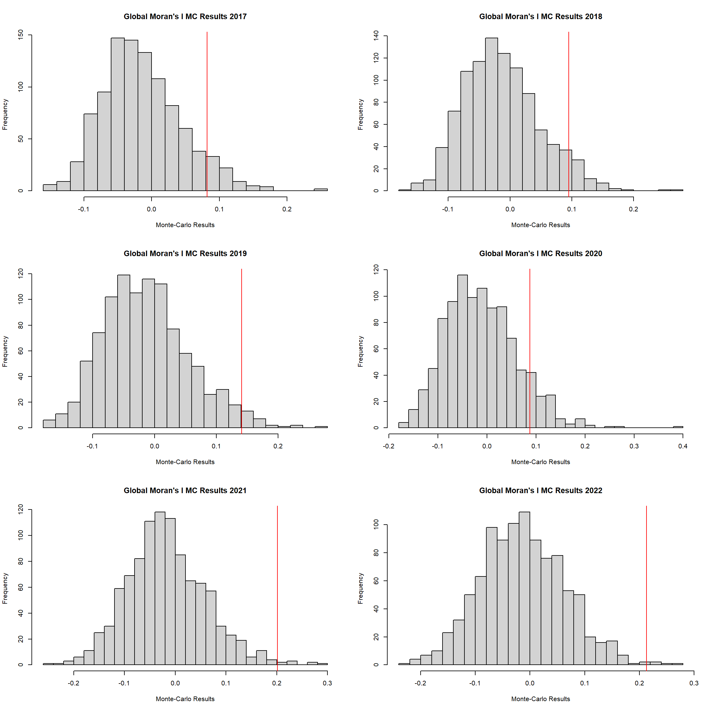
alternative hypothesis: greater

2.6.3 Global Moran’s I Permutation test

# List of gmoranMC objects for each year
gmoranMC_list <- list(gmoranMC_2017, gmoranMC_2018, gmoranMC_2019, 
                      gmoranMC_2020, gmoranMC_2021, gmoranMC_2022)

# Corresponding year labels for the titles
year_labels <- c("2017", "2018", "2019", "2020", "2021", "2022")

# Set up the plotting area to have 3 rows and 2 columns for the six histograms
par(mfrow = c(3, 2))

# Loop through each year and plot the histogram
for (i in 1:length(gmoranMC_list)) {
  gmoranMC <- gmoranMC_list[[i]]
  year <- year_labels[i]
  
  # Plot the histogram for the current year
  hist(gmoranMC$res, 
       main = paste("Global Moran's I MC Results", year), 
       breaks = 20,
       xlab = "Monte-Carlo Results", 
       ylab = "Frequency")
  
  # Add a vertical line for the observed Moran's I statistic
  abline(v = gmoranMC$statistic, col = "red")
}

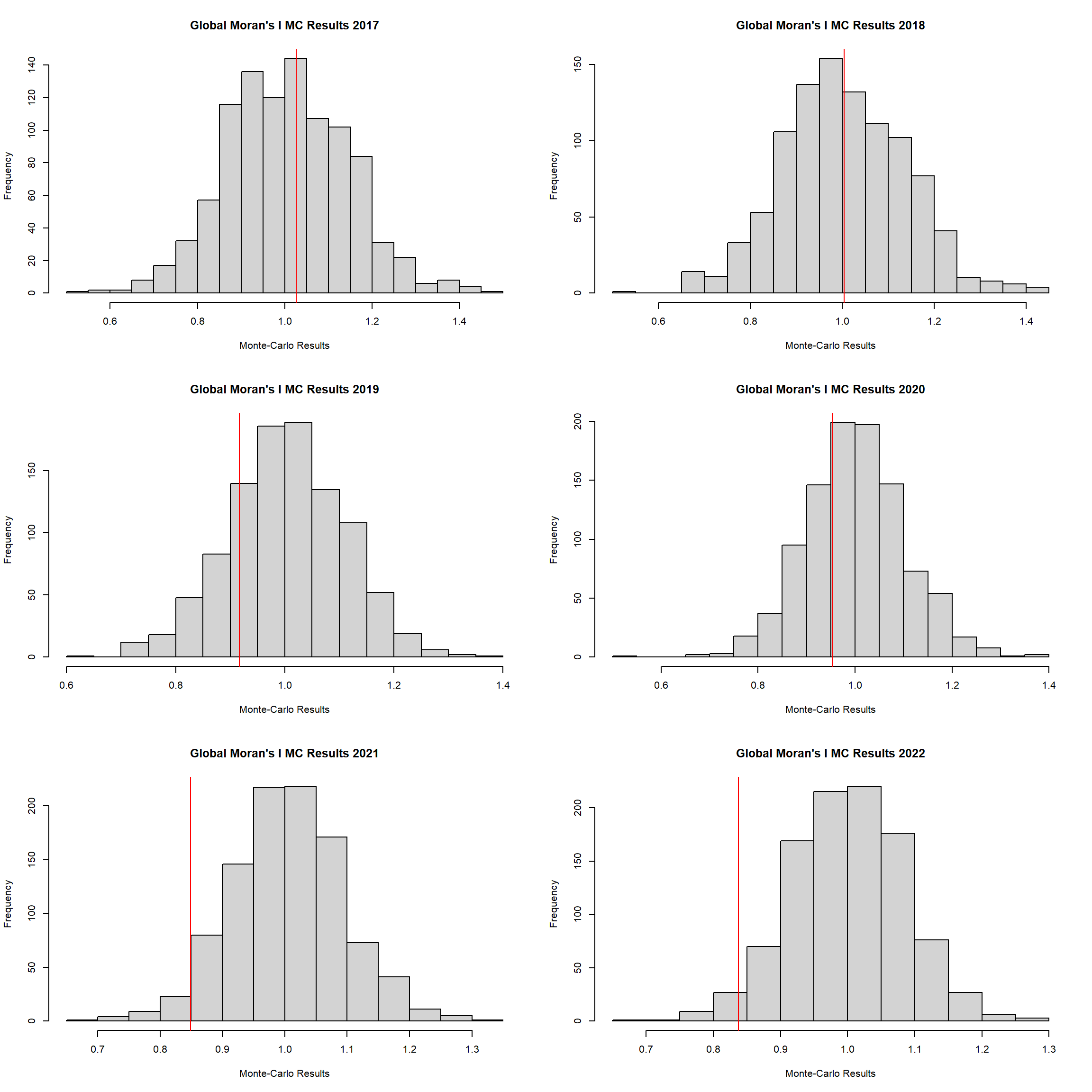
2.6.4 Global Geary’s C Permutation test

# List of bperm objects for each year
gmoranMC_list <- list(bperm_2017, bperm_2018, bperm_2019, 
                      bperm_2020, bperm_2021, bperm_2022)

# Corresponding year labels for the titles
year_labels <- c("2017", "2018", "2019", "2020", "2021", "2022")

# Set up the plotting area to have 3 rows and 2 columns for the six histograms
par(mfrow = c(3, 2))

# Loop through each year and plot the histogram
for (i in 1:length(gmoranMC_list)) {
  gmoranMC <- gmoranMC_list[[i]]
  year <- year_labels[i]
  
  # Plot the histogram for the current year
  hist(gmoranMC$res, 
       main = paste("Global Moran's I MC Results", year),
       breaks = 20,
       xlab = "Monte-Carlo Results", 
       ylab = "Frequency")
  
  # Add a vertical line for the observed Moran's I statistic
  abline(v = gmoranMC$statistic, col = "red")
}

2.6.5 Temporal Trends (2017-2022)

We can then analyze the spatial patterns of drug-related cases in Thailand over the period from 2017 to 2022 using Moran’s I and Geary’s C global spatial autocorrelation tests. The Moran’s I statistic identifies whether similar case values are clustered across regions, while Geary’s C focuses on local-level similarity, both crucial in understanding the distribution of drug-related offenses over time.

# Create a data frame to store Moran's I statistics and p-values
moran_i_results <- data.frame(
  Year = c(2017, 2018, 2019, 2020, 2021, 2022),
  Moran_I_Stat = c(global_moran_test_2017_statistics, global_moran_test_2018_statistics,
                   global_moran_test_2019_statistics, global_moran_test_2020_statistics,
                   global_moran_test_2021_statistics, global_moran_test_2022_statistics),
  Moran_I_p_value = c(global_moran_test_2017_p_value, global_moran_test_2018_p_value,
                      global_moran_test_2019_p_value, global_moran_test_2020_p_value,
                      global_moran_test_2021_p_value, global_moran_test_2022_p_value)
)

# Consolidate the Geary C test data into a data frame
geary_c_results <- data.frame(
  Year = c(2017, 2018, 2019, 2020, 2021, 2022),
  Geary_C_Stat = c(global_c_test_2017_statistics, global_c_test_2018_statistics, 
                   global_c_test_2019_statistics, global_c_test_2020_statistics, 
                   global_c_test_2021_statistics, global_c_test_2022_statistics),
  Geary_C_p_value = c(global_c_test_2017_p_value, global_c_test_2018_p_value, 
                      global_c_test_2019_p_value, global_c_test_2020_p_value, 
                      global_c_test_2021_p_value, global_c_test_2022_p_value)
)

Notes

Moran’s I (2017 - 2022) 2017: Moran’s I = 0.0821, p-value = 0.0577 2018: Moran’s I = 0.0952, p-value = 0.0423 2019: Moran’s I = 0.1410, p-value = 0.0149 2020: Moran’s I = 0.0875, p-value = 0.0835 2021: Moran’s I = 0.2013, p-value = 0.0024 2022: Moran’s I = 0.2133, p-value = 0.0015

Geary’s C (2017 - 2022) 2017: Geary’s C = 1.0258, p-value = 0.5714 2018: Geary’s C = 1.0037, p-value = 0.5106 2019: Geary’s C = 0.9167, p-value = 0.2260 2020: Geary’s C = 0.9528, p-value = 0.3234 2021: Geary’s C = 0.8489, p-value = 0.0433 2022: Geary’s C = 0.8377, p-value = 0.0292

# Plot Moran's I Statistic over the years
ggplot(moran_i_results, aes(x = Year, y = Moran_I_Stat)) +
  geom_line() + 
  geom_point() +
  labs(title = "Moran's I Statistic Trend (2017-2022)", 
       x = "Year", 
       y = "Moran's I Statistic") +
  theme_minimal()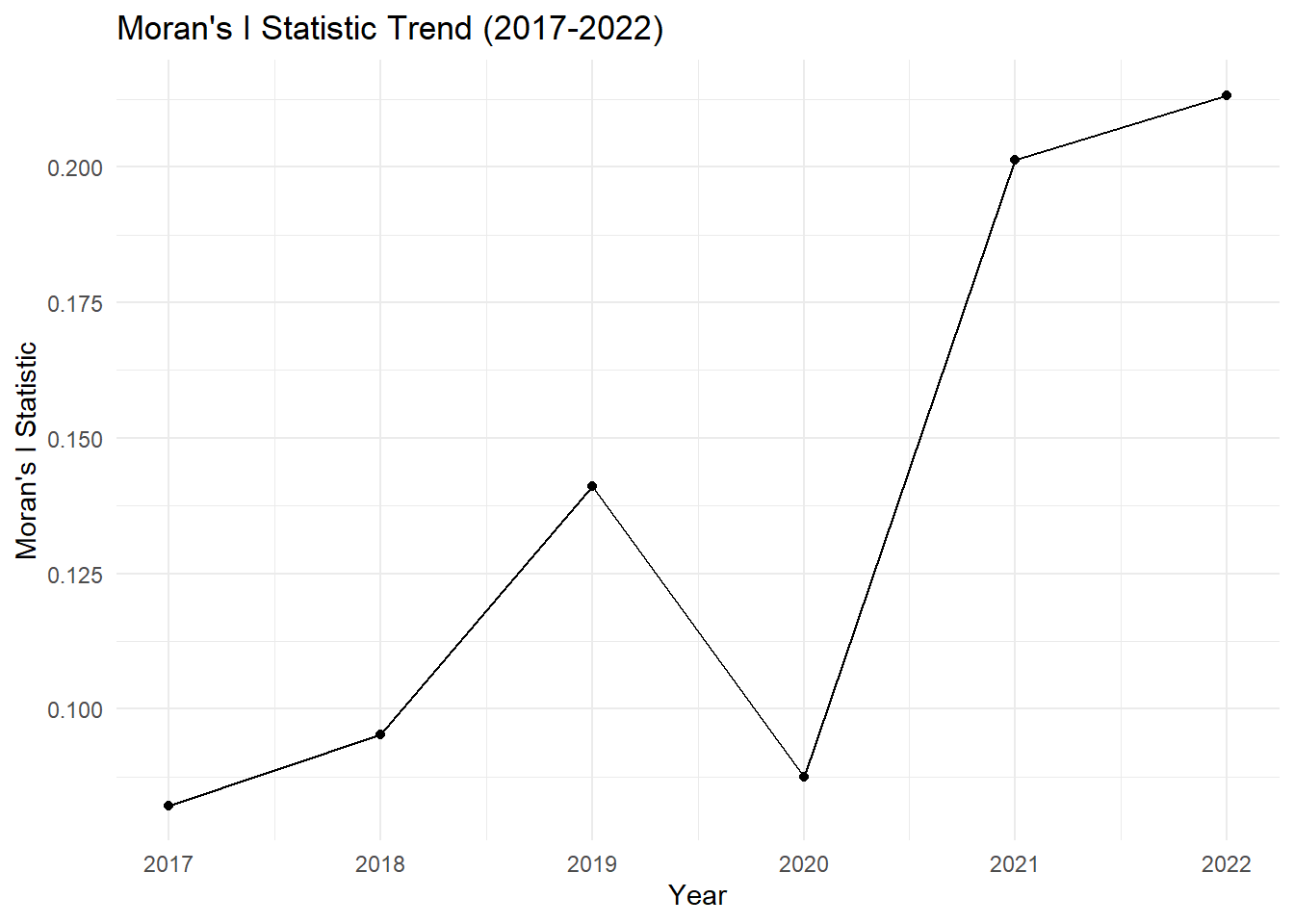

# Plot p-values over the years
ggplot(moran_i_results, aes(x = Year, y = Moran_I_p_value)) +
  geom_line() + 
  geom_point() +
  geom_hline(yintercept = 0.05, linetype = "dashed", color = "red") +  # Significance threshold
  labs(title = "Moran's I Test p-values (2017-2022)", 
       x = "Year", 
       y = "p-value") +
  theme_minimal()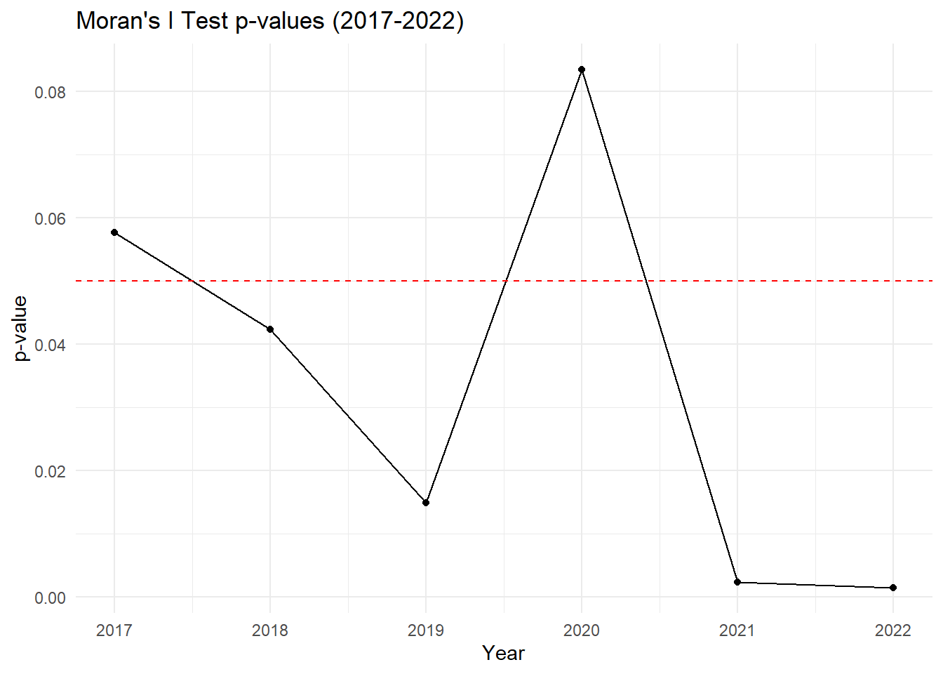

Reflection

Moran’s I (2017 - 2022)

2017: Moran’s I = 0.0821, p-value = 0.0577

2018: Moran’s I = 0.0952, p-value = 0.0423

2019: Moran’s I = 0.1410, p-value = 0.0149

2020: Moran’s I = 0.0875, p-value = 0.0835

2021: Moran’s I = 0.2013, p-value = 0.0024

2022: Moran’s I = 0.2133, p-value = 0.0015

Key Insights:

• 2017–2019: There is a gradual increase in spatial autocorrelation, with clustering becoming statistically significant by 2018 and peaking in 2019.

• 2020: A slight drop in Moran’s I indicates weaker spatial clustering, and the p-value suggests the autocorrelation is no longer significant. This could indicate that drug-related cases became more dispersed or random in 2020.

• 2021–2022: A sharp rise in Moran’s I shows that spatial clustering of drug-related cases became very strong in these years, and it is statistically significant with p-values well below 0.05. Drug-related cases are now highly concentrated in certain areas.

# Plot Geary C Statistic over the years
ggplot(geary_c_results, aes(x = Year, y = Geary_C_Stat)) +
  geom_line() + 
  geom_point() +
  labs(title = "Geary C Statistic Trend (2017-2022)", 
       x = "Year", 
       y = "Geary C Statistic") +
  theme_minimal()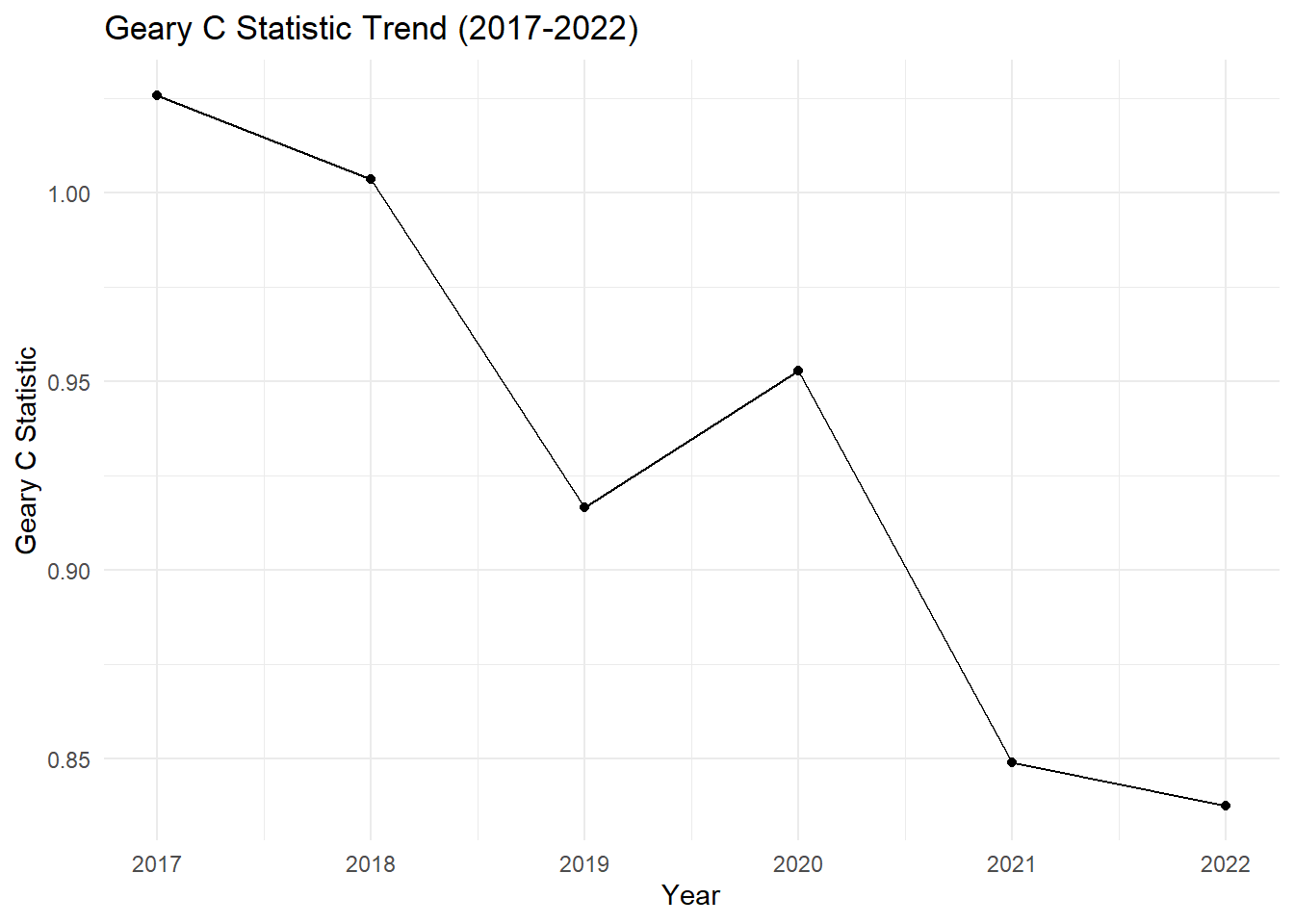

# Plot p-values over the years
ggplot(geary_c_results, aes(x = Year, y = Geary_C_p_value)) +
  geom_line() + 
  geom_point() +
  geom_hline(yintercept = 0.05, linetype = "dashed", color = "red") +  # Mark significance threshold
  labs(title = "Geary C Test p-values (2017-2022)", 
       x = "Year", 
       y = "p-value") +
  theme_minimal()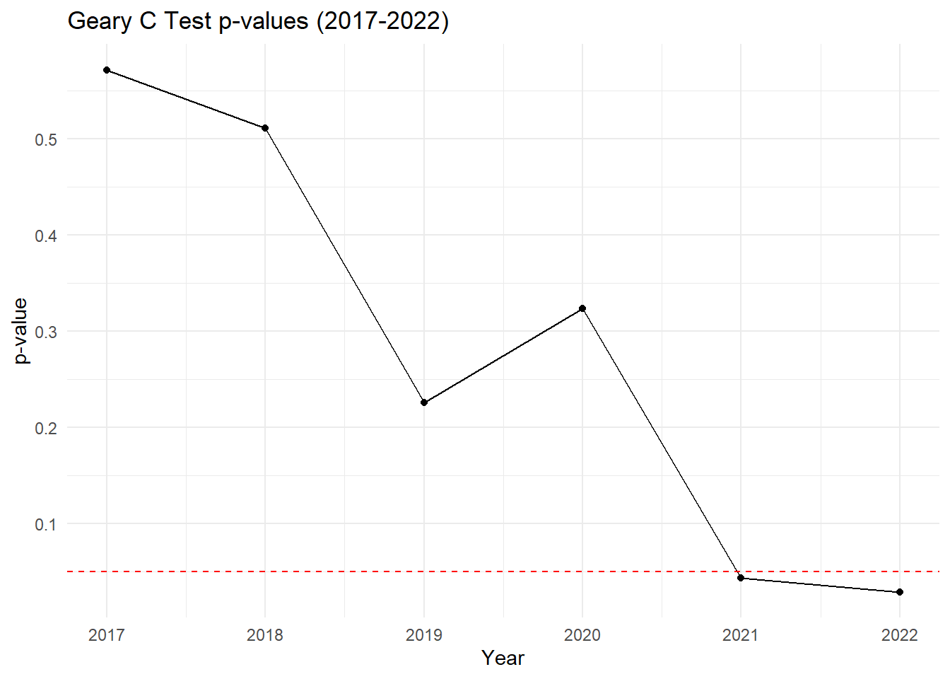

Reflection

Geary’s C (2017 - 2022)

2017: Geary’s C = 1.0258, p-value = 0.5714

2018: Geary’s C = 1.0037, p-value = 0.5106

2019: Geary’s C = 0.9167, p-value = 0.2260

2020: Geary’s C = 0.9528, p-value = 0.3234

2021: Geary’s C = 0.8489, p-value = 0.0433

2022: Geary’s C = 0.8377, p-value = 0.0292

Key Insights:

• 2017–2018: Geary’s C values are very close to 1, indicating no significant spatial autocorrelation, meaning the distribution of drug-related cases was largely random.

• 2019: The Geary’s C statistic starts to dip below 1, indicating emerging spatial autocorrelation, though it is not yet statistically significant.

• 2020: Geary’s C rises slightly, indicating a slight weakening of spatial autocorrelation, but the cases are still mostly random with no significant clustering.

• 2021–2022: A marked decrease in Geary’s C below 1, coupled with p-values dropping below 0.05, suggests significant clustering of similar values. This means that in the last two years, drug-related cases are no longer random and are now highly clustered.

2.6.6 Conclusion

From 2017 to 2022, both Moran’s I and Geary’s C statistics reveal an evolving spatial structure of drug-related cases. While earlier years exhibit weaker or random spatial patterns, by 2021 and 2022, significant clustering emerged, indicating an increase in spatial autocorrelation. This shift reflects that drug-related incidents are becoming more concentrated in specific areas, which could suggest targeted intervention zones for policy and law enforcement.

2.7 Local Measures of Spatial Autocorrelation

Building on the insights gained from global measures, local spatial autocorrelation focuses on identifying specific regions within the broader area that deviate from global trends. Techniques like Local Moran’s I allow for the detection of localized clusters and outliers, revealing spatial heterogeneity that might be masked by global statistics. This localized approach is crucial for pinpointing areas of high significance, enabling targeted interventions and more refined spatial decision-making.

2.7.1 Local Moran’s I

For each year from 2017 to 2022, Local Moran’s I is calculated for each province in Thailand. This involves assessing the spatial autocorrelation of drug use cases, and for each year, a statistical test is performed with 99 simulations to generate a p-value for significance testing. Provinces with a p-value below 0.05 are considered statistically significant, and the resulting spatial autocorrelation patterns are visualized. The results for each year are presented using maps showing both Local Moran’s I values and their corresponding p-values, followed by a final map that highlights only statistically significant clusters (p < 0.05). This iterative approach for multiple years enables the detection of persistent clusters of drug use cases across time, helping to identify long-term trends and regional patterns.

Year 2017

set.seed(4242)
lisa_2017 <- wm_q_2017 %>% 
  mutate(local_moran = local_moran(
    no_cases, nb, wt, nsim = 99),
         .before = 1) %>%
  unnest(local_moran)
lisa_2017

Simple feature collection with 77 features and 21 fields
Geometry type: MULTIPOLYGON
Dimension:     XY
Bounding box:  xmin: 97.34336 ymin: 5.613038 xmax: 105.637 ymax: 20.46507
Geodetic CRS:  WGS 84
# A tibble: 77 × 22
       ii        eii var_ii    z_ii          p_ii p_ii_sim p_folded_sim skewness
    <dbl>      <dbl>  <dbl>   <dbl>         <dbl>    <dbl>        <dbl>    <dbl>
 1 -0.556 -0.726     3.18    0.0955 0.924             0.84         0.42     1.15
 2  0.335  0.00121   0.110   1.01   0.314             0.06         0.03    -2.24
 3 -0.652  0.0429    0.0203 -4.87   0.00000109        0.04         0.02    -2.46
 4 -0.492 -0.0000714 0.0516 -2.17   0.0303            0.12         0.06    -2.22
 5  0.171  0.00626   0.0340  0.892  0.372             0.3          0.15    -1.52
 6  0.122 -0.00370   0.0132  1.09   0.276             0.06         0.03    -2.73
 7 -0.929  0.00822   0.0243 -6.00   0.00000000192     0.02         0.01    -3.07
 8  0.142 -0.00256   0.0784  0.516  0.606             0.58         0.29    -1.47
 9  0.329  0.00292   0.0827  1.13   0.256             0.04         0.02    -1.99
10  0.264  0.0694    0.0565  0.818  0.413             0.42         0.21    -2.03
# ℹ 67 more rows
# ℹ 14 more variables: kurtosis <dbl>, mean <fct>, median <fct>, pysal <fct>,
#   nb <nb>, wt <list>, fiscal_year <int>, types_of_drug_offenses <chr>,
#   no_cases <int>, province_en <chr>, Shape_Leng <dbl>, Shape_Area <dbl>,
#   date <date>, geometry <MULTIPOLYGON [°]>

Visualising Local Moran’s I_i

tm_shape(lisa_2017)+
  tm_fill("ii", 
          palette = c("#b7dce9","#e1ecbb","#f5f3a6",
                      "#f8d887","#ec9a64","#d21b1c"),
          title = "Local Moran's I",
          midpoint = NA,
          legend.hist = TRUE, 
          legend.is.portrait = TRUE,
          legend.hist.z = 0.1) +
  tm_borders(col = "black", alpha = 0.6)+
  tm_layout(main.title = "Province-level Spatial Autocorrelation \n of drug use cases in Thailand",
            main.title.position = "center",
            main.title.size = 1.7,
            main.title.fontface = "bold",
            legend.title.size = 1.8,
            legend.text.size = 1.3,
            frame = TRUE) +
  tm_borders(alpha = 0.5) +
  tm_compass(type="8star", text.size = 1.5, size = 3, position=c("RIGHT", "TOP")) +
  tm_scale_bar(position=c("LEFT", "BOTTOM"), text.size=1.2) +
  tm_grid(labels.size = 1,alpha =0.2)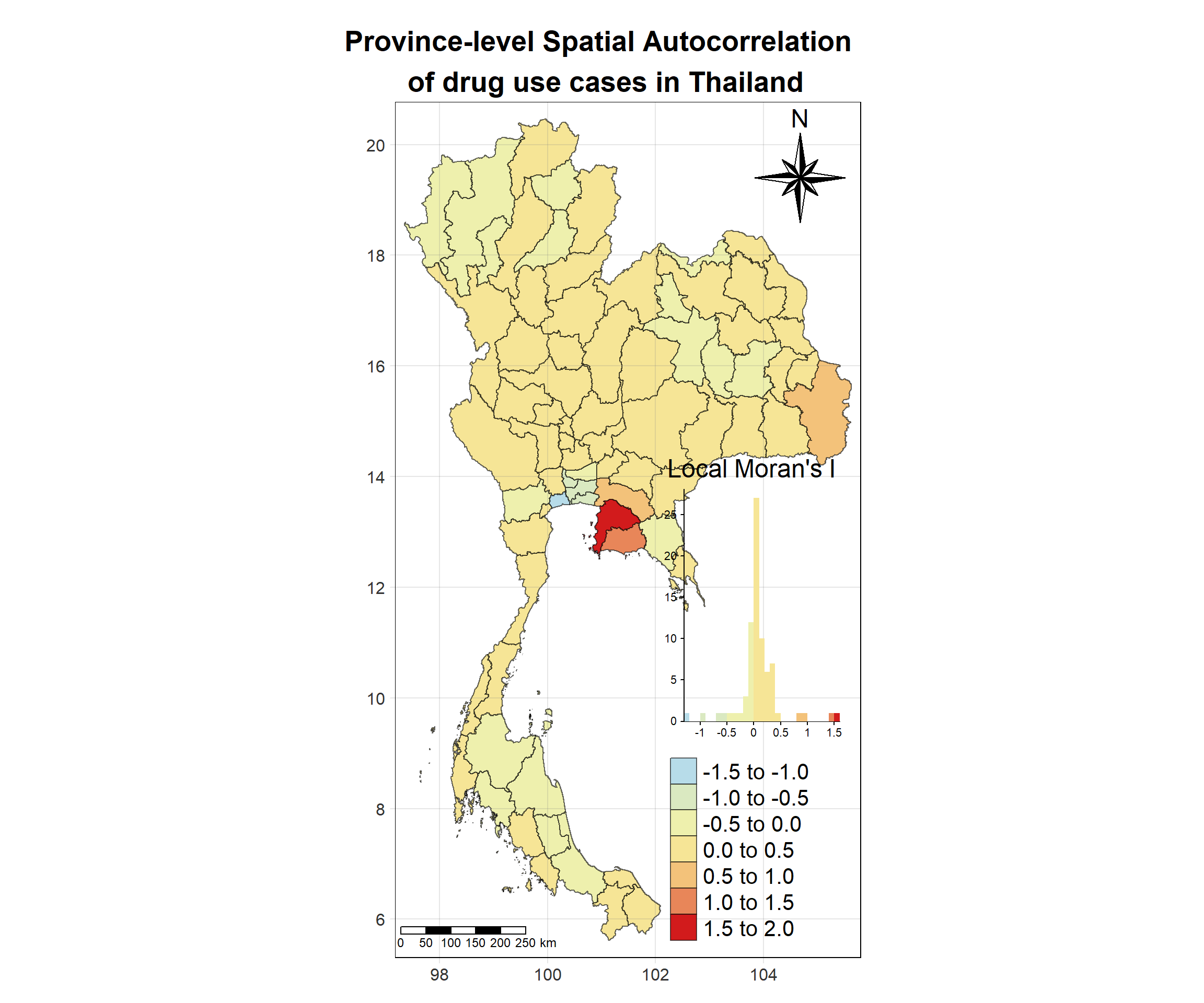

Visualising Local Moran’s I_i p-value

tm_shape(lisa_2017)+
  tm_fill("p_ii_sim", 
          palette = c("#b7dce9","#c9e3d2","#f5f3a6","#ec9a64","#d21b1c"),
          title = "p-value",
          midpoint = NA,
          legend.hist = TRUE, 
          legend.is.portrait = TRUE,
          legend.hist.z = 0.1) +
  tm_borders(col = "black", alpha = 0.6)+
  tm_layout(main.title = "Statistical Significance of Spatial \n Autocorrelation of drug use cases in Thailand",
            main.title.position = "center",
            main.title.size = 1.7,
            main.title.fontface = "bold",
            legend.title.size = 1.8,
            legend.text.size = 1.3,
            frame = TRUE) +
  tm_borders(alpha = 0.5) +
  tm_compass(type="8star", text.size = 1.5, size = 3, position=c("RIGHT", "TOP")) +
  tm_scale_bar(position=c("LEFT", "BOTTOM"), text.size=1.2) +
  tm_grid(labels.size = 1,alpha =0.2)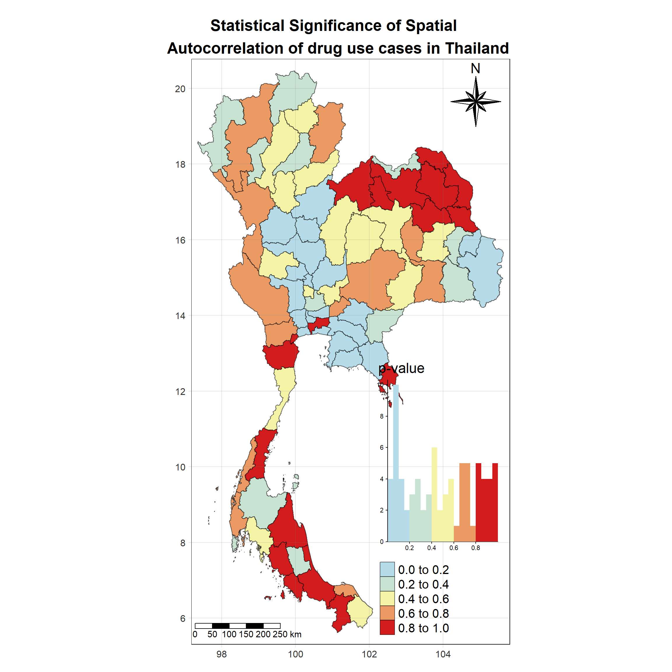

Visualising Statistically Significant Local Spatial Autocorrelation Map

lisa_2017_sig <- lisa_2017  %>%
  filter(p_ii_sim < 0.05) %>% mutate(label = province_en)

tm_shape(lisa_2017)+
  tm_polygons() +
  tm_borders(col = "black", alpha = 0.6)+
tm_shape(lisa_2017_sig)+
  tm_fill("ii", 
          palette = c("#b7dce9","#e1ecbb","#f5f3a6",
                      "#f8d887","#ec9a64","#d21b1c"),
          breaks = c(0, 0.001, 0.01, 0.05, 1),
          labels = c("0.001", "0.01", "0.05", "Not sig"),
          title = "Local Moran's I (p < 0.05)",
          midpoint = NA,
          legend.hist = TRUE, 
          legend.is.portrait = TRUE,
          legend.hist.z = 0.1) +
  tm_borders(col = "black", alpha = 0.6)+
  tm_layout(main.title = "Statistically Significant Village-Level Spatial \n Autocorrelation Map of drug use cases \n in Thailand",
            main.title.position = "center",
            main.title.size = 1.7,
            main.title.fontface = "bold",
            legend.title.size = 1.8,
            legend.text.size = 1.3,
            frame = TRUE) +
  tm_borders(alpha = 0.5) +
  tm_compass(type="8star", text.size = 1.5, size = 3, position=c("RIGHT", "TOP")) +
  tm_scale_bar(position=c("LEFT", "BOTTOM"), text.size=1.2) +
  tm_grid(labels.size = 1,alpha =0.2)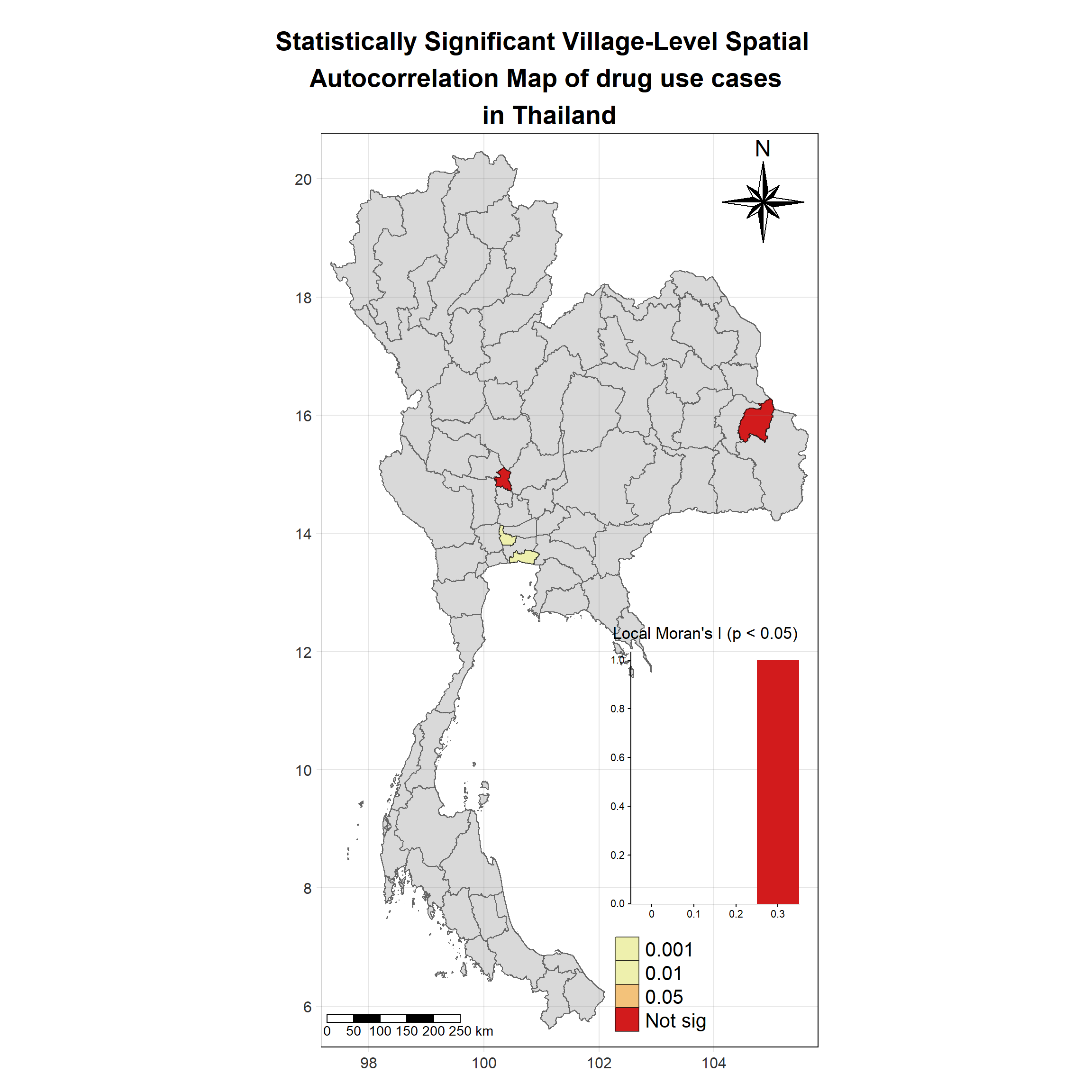

Year 2018

set.seed(4242)
lisa_2018 <- wm_q_2018 %>% 
  mutate(local_moran = local_moran(
    no_cases, nb, wt, nsim = 99),
         .before = 1) %>%
  unnest(local_moran)
lisa_2018

Simple feature collection with 77 features and 21 fields
Geometry type: MULTIPOLYGON
Dimension:     XY
Bounding box:  xmin: 97.34336 ymin: 5.613038 xmax: 105.637 ymax: 20.46507
Geodetic CRS:  WGS 84
# A tibble: 77 × 22
         ii       eii    var_ii   z_ii       p_ii p_ii_sim p_folded_sim skewness
      <dbl>     <dbl>     <dbl>  <dbl>      <dbl>    <dbl>        <dbl>    <dbl>
 1  0.192   -0.708    3.37       0.490    6.24e-1     0.62         0.31     1.16
 2  0.358    0.00374  0.130      0.984    3.25e-1     0.16         0.08    -1.86
 3 -0.188    0.0101   0.00188   -4.57     4.85e-6     0.04         0.02    -2.20
 4 -0.0355   0.000684 0.000313  -2.04     4.11e-2     0.14         0.07    -2.21
 5  0.0580   0.00852  0.0157     0.395    6.93e-1     0.84         0.42    -1.30
 6  0.00332 -0.000511 0.0000984  0.387    6.99e-1     0.76         0.38    -2.42
 7  1.74    -0.00597  0.122      5.00     5.82e-7     0.04         0.02     2.73
 8 -0.0724  -0.0104   0.0568    -0.260    7.95e-1     0.64         0.32    -1.59
 9  0.280    0.0107   0.0816     0.943    3.46e-1     0.22         0.11    -1.72
10  0.178    0.0436   0.0545     0.573    5.66e-1     0.66         0.33    -1.63
# ℹ 67 more rows
# ℹ 14 more variables: kurtosis <dbl>, mean <fct>, median <fct>, pysal <fct>,
#   nb <nb>, wt <list>, fiscal_year <int>, types_of_drug_offenses <chr>,
#   no_cases <int>, province_en <chr>, Shape_Leng <dbl>, Shape_Area <dbl>,
#   date <date>, geometry <MULTIPOLYGON [°]>

Visualising Local Moran’s I_i

tm_shape(lisa_2018)+
  tm_fill("ii", 
          palette = c("#b7dce9","#e1ecbb","#f5f3a6",
                      "#f8d887","#ec9a64","#d21b1c"),
          title = "Local Moran's I",
          midpoint = NA,
          legend.hist = TRUE, 
          legend.is.portrait = TRUE,
          legend.hist.z = 0.1) +
  tm_borders(col = "black", alpha = 0.6)+
  tm_layout(main.title = "Province-level Spatial Autocorrelation \n of drug use cases in Thailand",
            main.title.position = "center",
            main.title.size = 1.7,
            main.title.fontface = "bold",
            legend.title.size = 1.8,
            legend.text.size = 1.3,
            frame = TRUE) +
  tm_borders(alpha = 0.5) +
  tm_compass(type="8star", text.size = 1.5, size = 3, position=c("RIGHT", "TOP")) +
  tm_scale_bar(position=c("LEFT", "BOTTOM"), text.size=1.2) +
  tm_grid(labels.size = 1,alpha =0.2)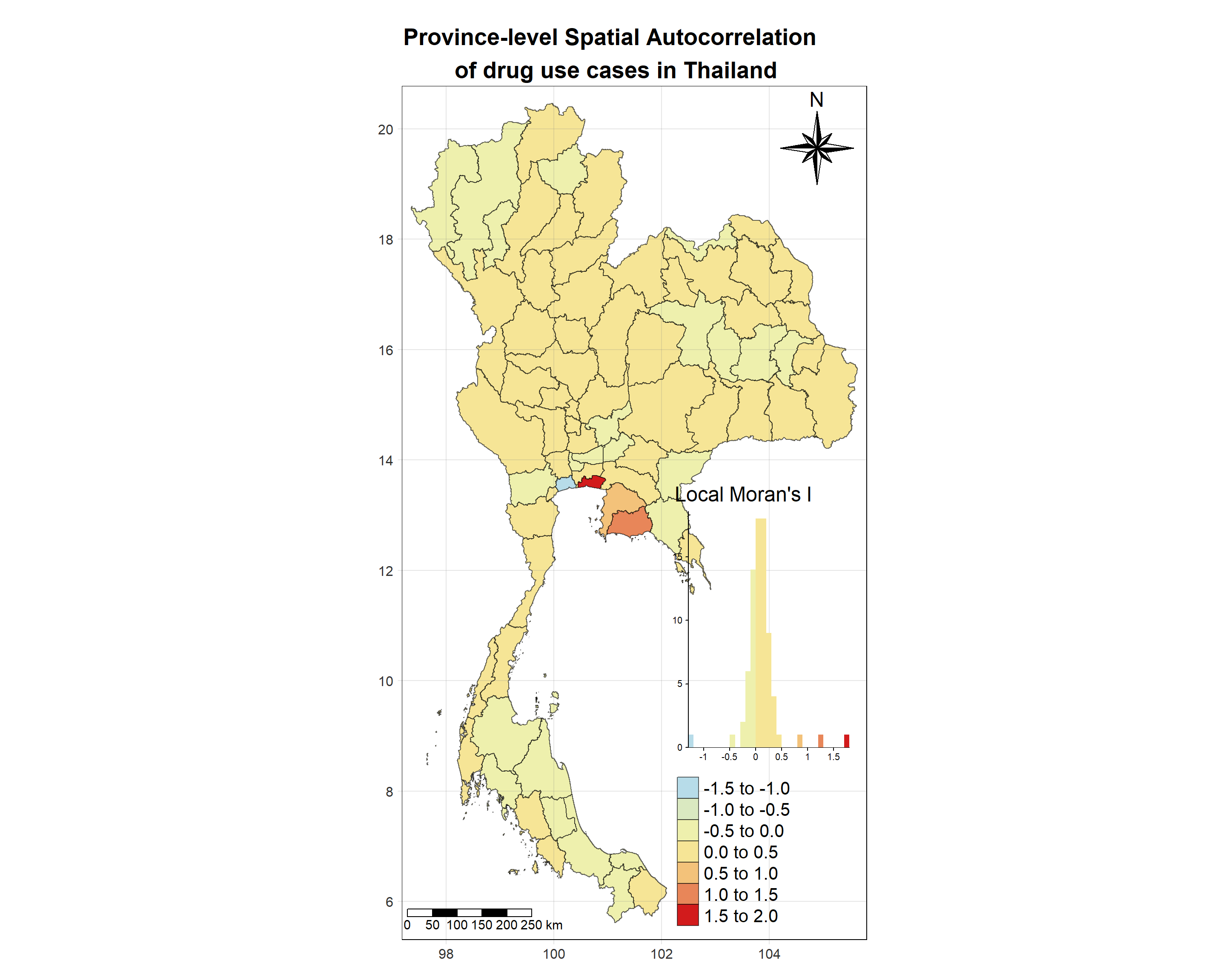

Visualising Local Moran’s I_i p-value

tm_shape(lisa_2018)+
  tm_fill("p_ii_sim", 
          palette = c("#b7dce9","#c9e3d2","#f5f3a6","#ec9a64","#d21b1c"),
          title = "p-value",
          midpoint = NA,
          legend.hist = TRUE, 
          legend.is.portrait = TRUE,
          legend.hist.z = 0.1) +
  tm_borders(col = "black", alpha = 0.6)+
  tm_layout(main.title = "Statistical Significance of Spatial \n Autocorrelation of drug use cases in Thailand",
            main.title.position = "center",
            main.title.size = 1.7,
            main.title.fontface = "bold",
            legend.title.size = 1.8,
            legend.text.size = 1.3,
            frame = TRUE) +
  tm_borders(alpha = 0.5) +
  tm_compass(type="8star", text.size = 1.5, size = 3, position=c("RIGHT", "TOP")) +
  tm_scale_bar(position=c("LEFT", "BOTTOM"), text.size=1.2) +
  tm_grid(labels.size = 1,alpha =0.2)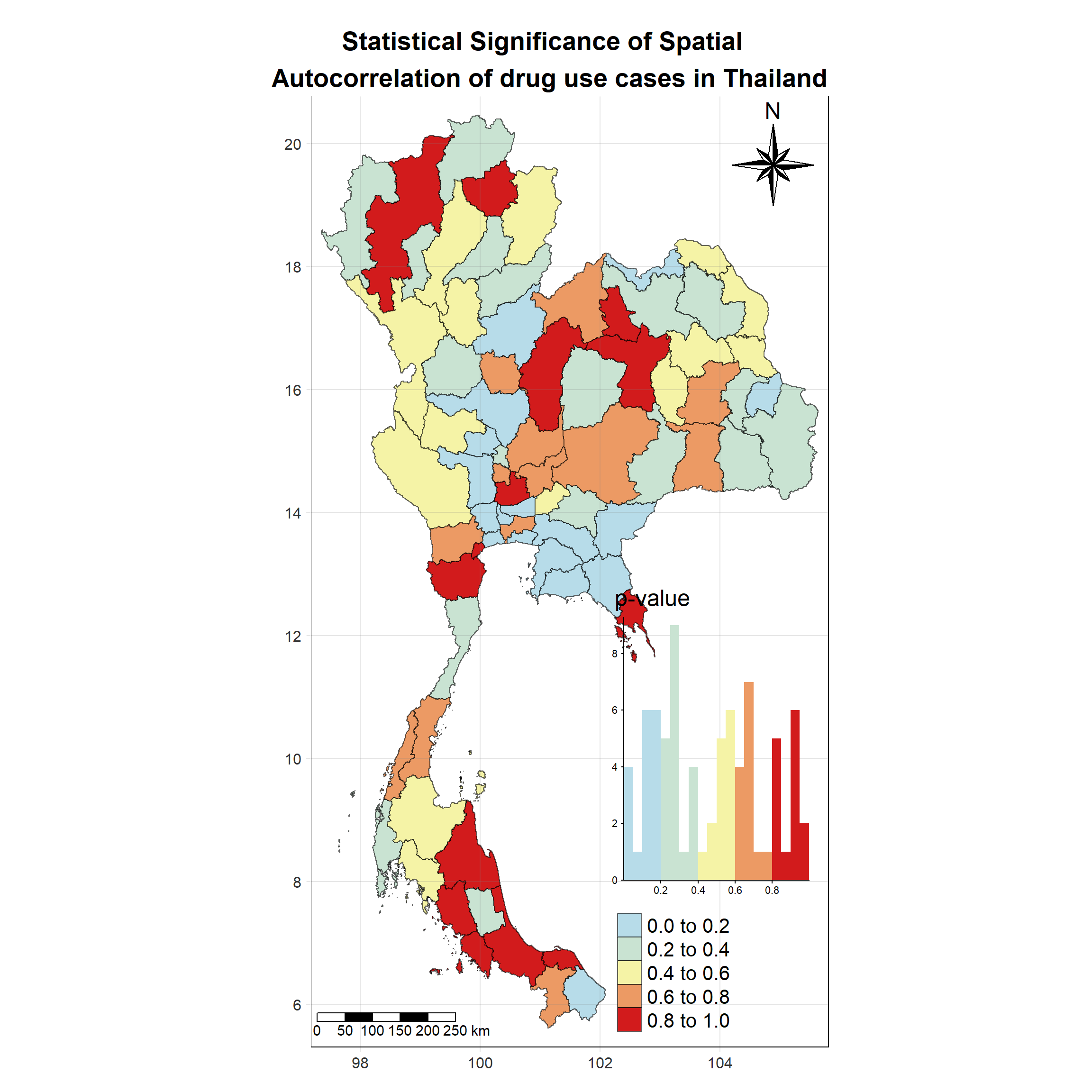

Visualising Statistically Significant Local Spatial Autocorrelation Map

lisa_2018_sig <- lisa_2018  %>%
  filter(p_ii_sim < 0.05) %>% mutate(label = province_en)

tm_shape(lisa_2018)+
  tm_polygons() +
  tm_borders(col = "black", alpha = 0.6)+
tm_shape(lisa_2018_sig)+
  tm_fill("ii", 
          palette = c("#b7dce9","#e1ecbb","#f5f3a6",
                      "#f8d887","#ec9a64","#d21b1c"),
          breaks = c(0, 0.001, 0.01, 0.05, 1),
          labels = c("0.001", "0.01", "0.05", "Not sig"),
          title = "Local Moran's I (p < 0.05)",
          midpoint = NA,
          legend.hist = TRUE, 
          legend.is.portrait = TRUE,
          legend.hist.z = 0.1) +
  tm_borders(col = "black", alpha = 0.6)+
  tm_layout(main.title = "Statistically Significant Village-Level Spatial \n Autocorrelation Map of drug use cases \n in Thailand",
            main.title.position = "center",
            main.title.size = 1.7,
            main.title.fontface = "bold",
            legend.title.size = 1.8,
            legend.text.size = 1.3,
            frame = TRUE) +
  tm_borders(alpha = 0.5) +
  tm_compass(type="8star", text.size = 1.5, size = 3, position=c("RIGHT", "TOP")) +
  tm_scale_bar(position=c("LEFT", "BOTTOM"), text.size=1.2) +
  tm_grid(labels.size = 1,alpha =0.2)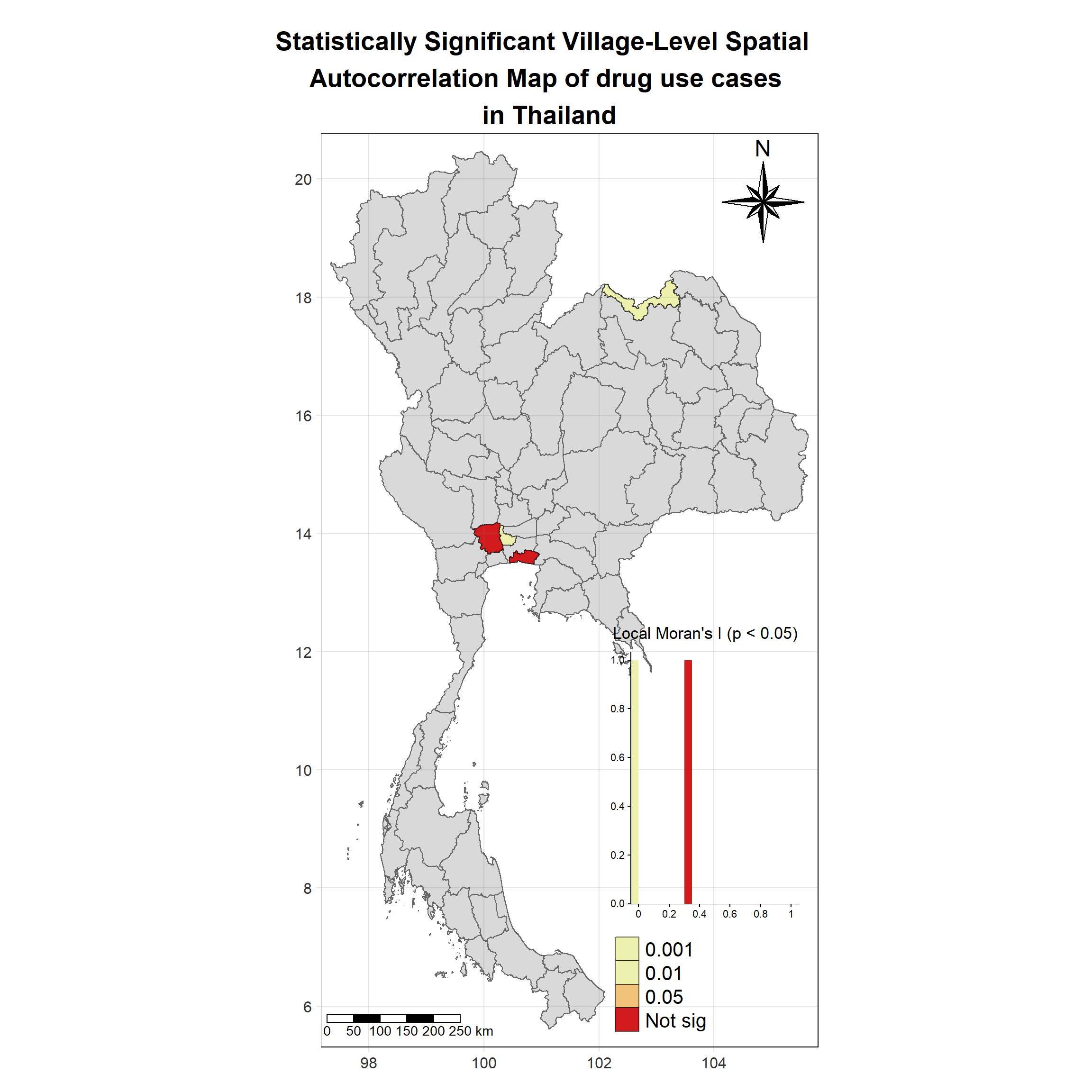

Year 2019

set.seed(4242)
lisa_2019 <- wm_q_2019 %>% 
  mutate(local_moran = local_moran(
    no_cases, nb, wt, nsim = 99),
         .before = 1) %>%
  unnest(local_moran)
lisa_2019

Simple feature collection with 77 features and 21 fields
Geometry type: MULTIPOLYGON
Dimension:     XY
Bounding box:  xmin: 97.34336 ymin: 5.613038 xmax: 105.637 ymax: 20.46507
Geodetic CRS:  WGS 84
# A tibble: 77 × 22
          ii       eii    var_ii    z_ii     p_ii p_ii_sim p_folded_sim skewness
       <dbl>     <dbl>     <dbl>   <dbl>    <dbl>    <dbl>        <dbl>    <dbl>
 1  0.341    -0.478    3.34       0.448  0.654        0.6          0.3     1.09 
 2  0.306    -0.000190 0.0941     0.997  0.319        0.18         0.09   -1.30 
 3 -0.371     0.0183   0.0126    -3.47   0.000528     0.06         0.03   -1.64 
 4  0.216    -0.0101   0.0188     1.65   0.0991       0.18         0.09    1.64 
 5 -0.0149   -0.00255  0.000641  -0.488  0.625        0.76         0.38    0.733
 6 -0.000229 -0.000528 0.0000344  0.0510 0.959        0.9          0.45   -1.78 
 7  2.73      0.00364  0.517      3.79   0.000154     0.04         0.02    1.67 
 8 -0.270    -0.0190   0.0714    -0.938  0.348        0.3          0.15   -1.21 
 9  0.318     0.0122   0.0941     0.998  0.318        0.2          0.1    -1.15 
10  0.166     0.0420   0.107      0.379  0.704        0.94         0.47   -1.13 
# ℹ 67 more rows
# ℹ 14 more variables: kurtosis <dbl>, mean <fct>, median <fct>, pysal <fct>,
#   nb <nb>, wt <list>, fiscal_year <int>, types_of_drug_offenses <chr>,
#   no_cases <int>, province_en <chr>, Shape_Leng <dbl>, Shape_Area <dbl>,
#   date <date>, geometry <MULTIPOLYGON [°]>

Visualising Local Moran’s I_i

tm_shape(lisa_2019)+
  tm_fill("ii", 
          palette = c("#b7dce9","#e1ecbb","#f5f3a6",
                      "#f8d887","#ec9a64","#d21b1c"),
          title = "Local Moran's I",
          midpoint = NA,
          legend.hist = TRUE, 
          legend.is.portrait = TRUE,
          legend.hist.z = 0.1) +
  tm_borders(col = "black", alpha = 0.6)+
  tm_layout(main.title = "Province-level Spatial Autocorrelation \n of drug use cases in Thailand",
            main.title.position = "center",
            main.title.size = 1.7,
            main.title.fontface = "bold",
            legend.title.size = 1.8,
            legend.text.size = 1.3,
            frame = TRUE) +
  tm_borders(alpha = 0.5) +
  tm_compass(type="8star", text.size = 1.5, size = 3, position=c("RIGHT", "TOP")) +
  tm_scale_bar(position=c("LEFT", "BOTTOM"), text.size=1.2) +
  tm_grid(labels.size = 1,alpha =0.2)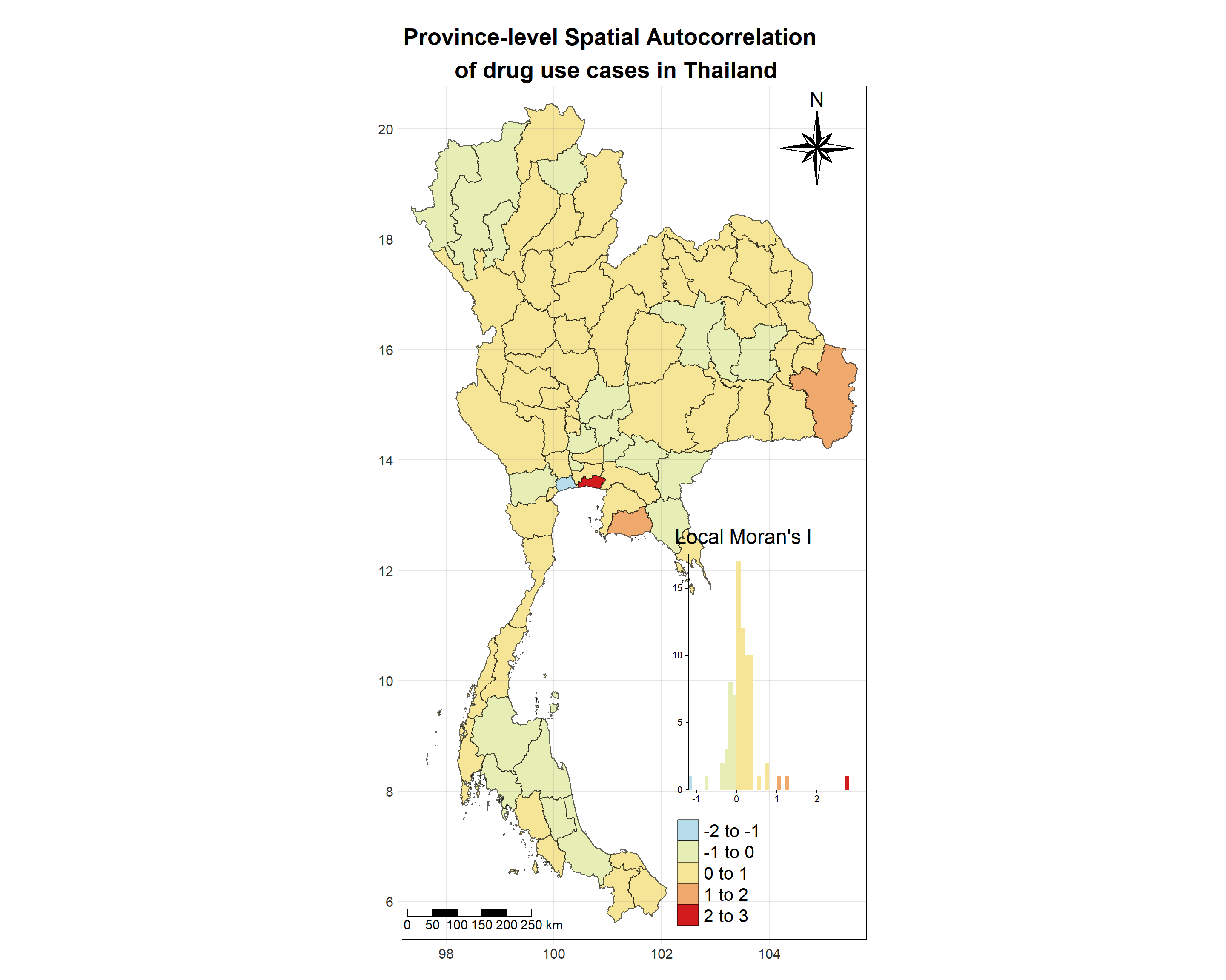

Visualising Local Moran’s I_i p-value

tm_shape(lisa_2019)+
  tm_fill("p_ii_sim", 
          palette = c("#b7dce9","#c9e3d2","#f5f3a6","#ec9a64","#d21b1c"),
          title = "p-value",
          midpoint = NA,
          legend.hist = TRUE, 
          legend.is.portrait = TRUE,
          legend.hist.z = 0.1) +
  tm_borders(col = "black", alpha = 0.6)+
  tm_layout(main.title = "Statistical Significance of Spatial \n Autocorrelation of drug use cases in Thailand",
            main.title.position = "center",
            main.title.size = 1.7,
            main.title.fontface = "bold",
            legend.title.size = 1.8,
            legend.text.size = 1.3,
            frame = TRUE) +
  tm_borders(alpha = 0.5) +
  tm_compass(type="8star", text.size = 1.5, size = 3, position=c("RIGHT", "TOP")) +
  tm_scale_bar(position=c("LEFT", "BOTTOM"), text.size=1.2) +
  tm_grid(labels.size = 1,alpha =0.2)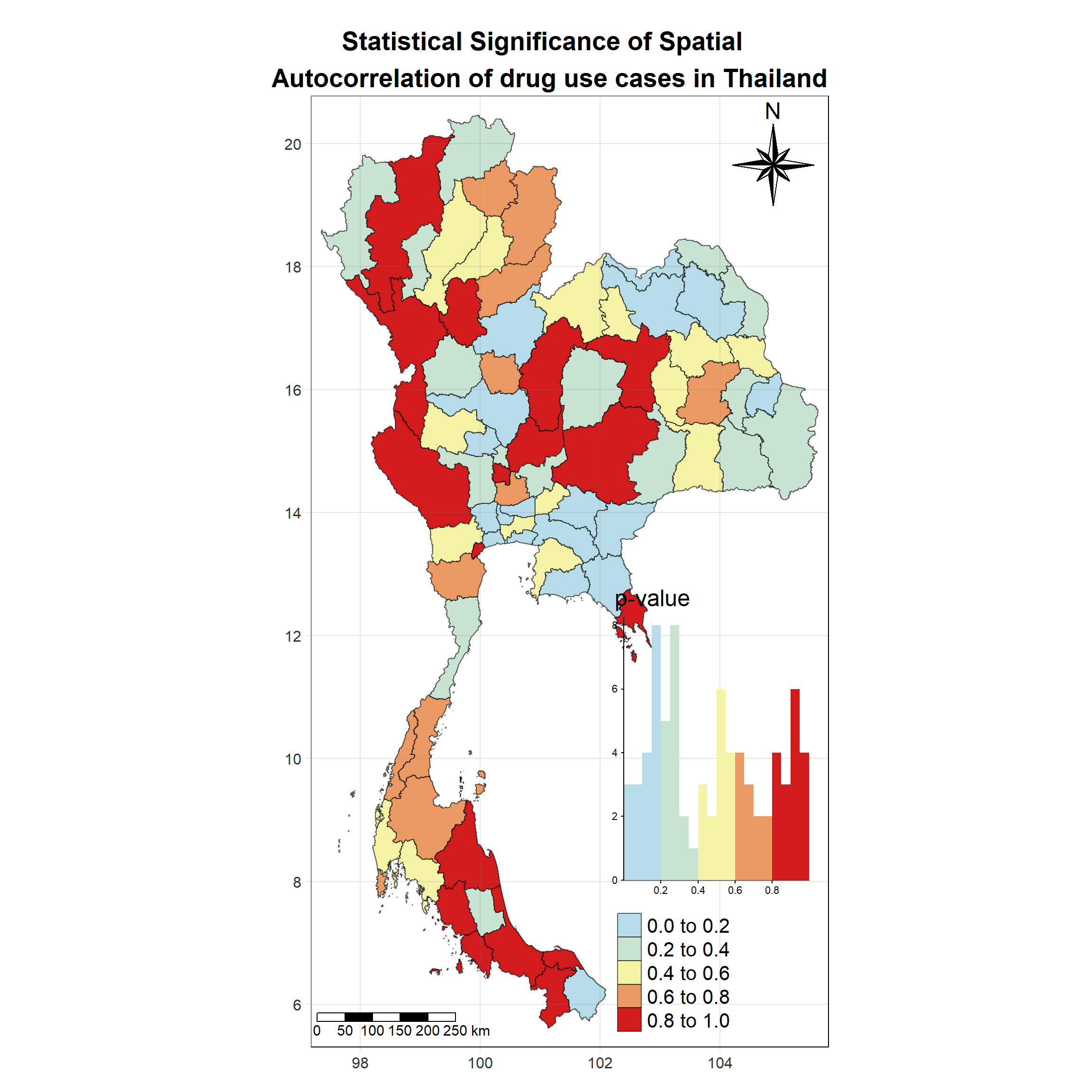

Visualising Statistically Significant Local Spatial Autocorrelation Map

lisa_2019_sig <- lisa_2019  %>%
  filter(p_ii_sim < 0.05) %>% mutate(label = province_en)

tm_shape(lisa_2019)+
  tm_polygons() +
  tm_borders(col = "black", alpha = 0.6)+
tm_shape(lisa_2019_sig)+
  tm_fill("ii", 
          palette = c("#b7dce9","#e1ecbb","#f5f3a6",
                      "#f8d887","#ec9a64","#d21b1c"),
          breaks = c(0, 0.001, 0.01, 0.05, 1),
          labels = c("0.001", "0.01", "0.05", "Not sig"),
          title = "Local Moran's I (p < 0.05)",
          midpoint = NA,
          legend.hist = TRUE, 
          legend.is.portrait = TRUE,
          legend.hist.z = 0.1) +
  tm_borders(col = "black", alpha = 0.6)+
  tm_layout(main.title = "Statistically Significant Village-Level Spatial \n Autocorrelation Map of drug use cases \n in Thailand",
            main.title.position = "center",
            main.title.size = 1.7,
            main.title.fontface = "bold",
            legend.title.size = 1.8,
            legend.text.size = 1.3,
            frame = TRUE) +
  tm_borders(alpha = 0.5) +
  tm_compass(type="8star", text.size = 1.5, size = 3, position=c("RIGHT", "TOP")) +
  tm_scale_bar(position=c("LEFT", "BOTTOM"), text.size=1.2) +
  tm_grid(labels.size = 1,alpha =0.2)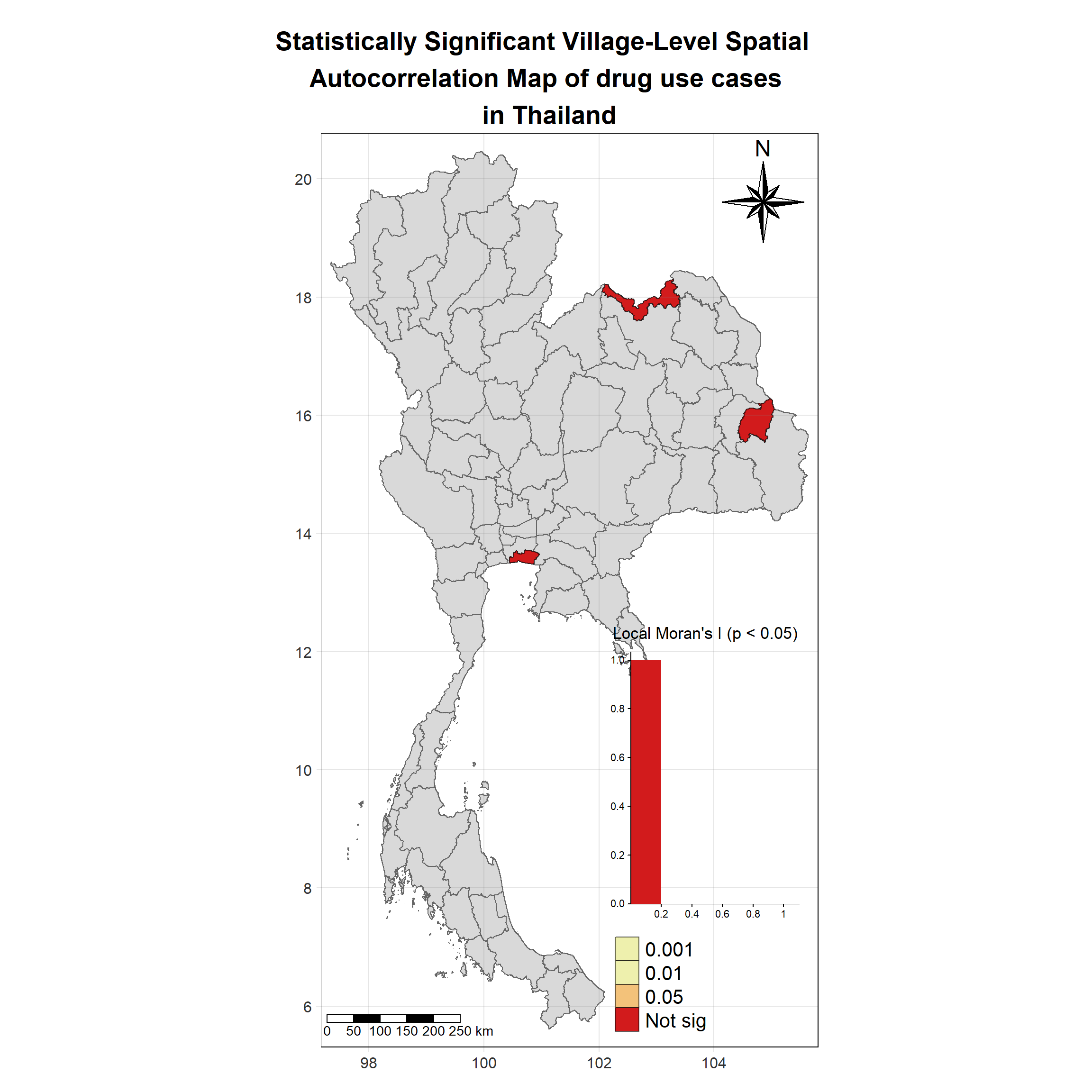

Year 2020

set.seed(4242)
lisa_2020 <- wm_q_2020 %>% 
  mutate(local_moran = local_moran(
    no_cases, nb, wt, nsim = 99),
         .before = 1) %>%
  unnest(local_moran)
lisa_2020

Simple feature collection with 77 features and 21 fields
Geometry type: MULTIPOLYGON
Dimension:     XY
Bounding box:  xmin: 97.34336 ymin: 5.613038 xmax: 105.637 ymax: 20.46507
Geodetic CRS:  WGS 84
# A tibble: 77 × 22
        ii       eii   var_ii    z_ii  p_ii p_ii_sim p_folded_sim skewness
     <dbl>     <dbl>    <dbl>   <dbl> <dbl>    <dbl>        <dbl>    <dbl>
 1 -0.0216 -0.0130   0.0485   -0.0392 0.969     0.82         0.41   -0.977
 2 -0.0896 -0.0233   0.0160   -0.524  0.600     0.76         0.38    0.955
 3 -0.0366 -0.000725 0.00435  -0.543  0.587     0.84         0.42    0.587
 4  0.0565 -0.0138   0.0512    0.310  0.756     0.9          0.45   -0.699
 5  0.0349 -0.0253   0.0500    0.269  0.788     0.92         0.46   -0.821
 6  0.0160  0.000767 0.000482  0.692  0.489     0.6          0.3    -0.828
 7 -0.121   0.0814   0.240    -0.413  0.680     0.54         0.27   -1.55 
 8  0.0184 -0.000515 0.00185   0.441  0.659     0.86         0.43   -1.19 
 9  1.52    0.0979   1.16      1.32   0.188     0.26         0.13    1.48 
10  0.325  -0.106    1.30      0.377  0.706     0.62         0.31    0.841
# ℹ 67 more rows
# ℹ 14 more variables: kurtosis <dbl>, mean <fct>, median <fct>, pysal <fct>,
#   nb <nb>, wt <list>, fiscal_year <int>, types_of_drug_offenses <chr>,
#   no_cases <int>, province_en <chr>, Shape_Leng <dbl>, Shape_Area <dbl>,
#   date <date>, geometry <MULTIPOLYGON [°]>

Visualising Local Moran’s I_i

tm_shape(lisa_2020)+
  tm_fill("ii", 
          palette = c("#b7dce9","#e1ecbb","#f5f3a6",
                      "#f8d887","#ec9a64","#d21b1c"),
          title = "Local Moran's I",
          midpoint = NA,
          legend.hist = TRUE, 
          legend.is.portrait = TRUE,
          legend.hist.z = 0.1) +
  tm_borders(col = "black", alpha = 0.6)+
  tm_layout(main.title = "Province-level Spatial Autocorrelation \n of drug use cases in Thailand",
            main.title.position = "center",
            main.title.size = 1.7,
            main.title.fontface = "bold",
            legend.title.size = 1.8,
            legend.text.size = 1.3,
            frame = TRUE) +
  tm_borders(alpha = 0.5) +
  tm_compass(type="8star", text.size = 1.5, size = 3, position=c("RIGHT", "TOP")) +
  tm_scale_bar(position=c("LEFT", "BOTTOM"), text.size=1.2) +
  tm_grid(labels.size = 1,alpha =0.2)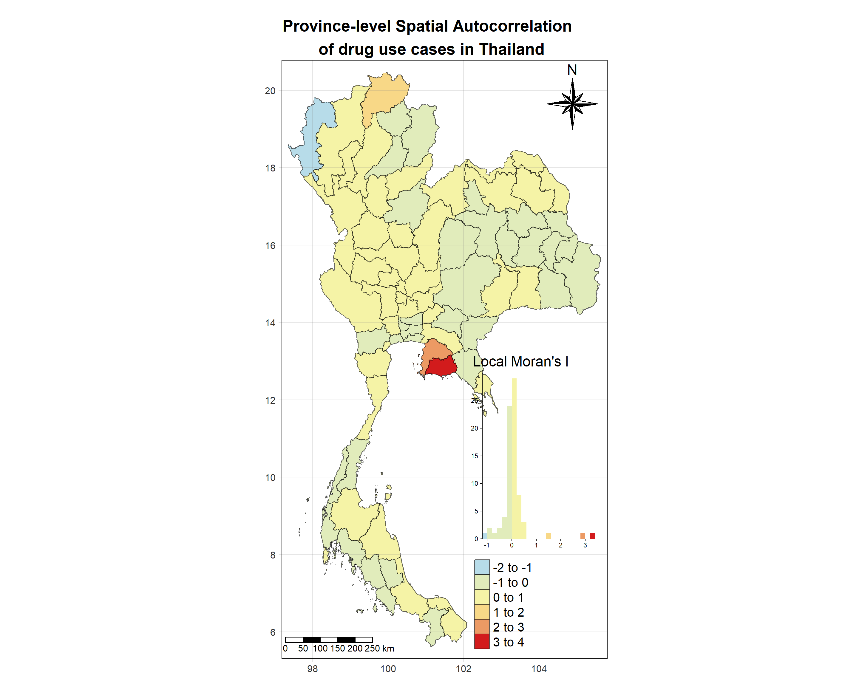

Visualising Local Moran’s I_i p-value

tm_shape(lisa_2020)+
  tm_fill("p_ii_sim", 
          palette = c("#b7dce9","#c9e3d2","#f5f3a6","#ec9a64","#d21b1c"),
          title = "p-value",
          midpoint = NA,
          legend.hist = TRUE, 
          legend.is.portrait = TRUE,
          legend.hist.z = 0.1) +
  tm_borders(col = "black", alpha = 0.6)+
  tm_layout(main.title = "Statistical Significance of Spatial \n Autocorrelation of drug use cases in Thailand",
            main.title.position = "center",
            main.title.size = 1.7,
            main.title.fontface = "bold",
            legend.title.size = 1.8,
            legend.text.size = 1.3,
            frame = TRUE) +
  tm_borders(alpha = 0.5) +
  tm_compass(type="8star", text.size = 1.5, size = 3, position=c("RIGHT", "TOP")) +
  tm_scale_bar(position=c("LEFT", "BOTTOM"), text.size=1.2) +
  tm_grid(labels.size = 1,alpha =0.2)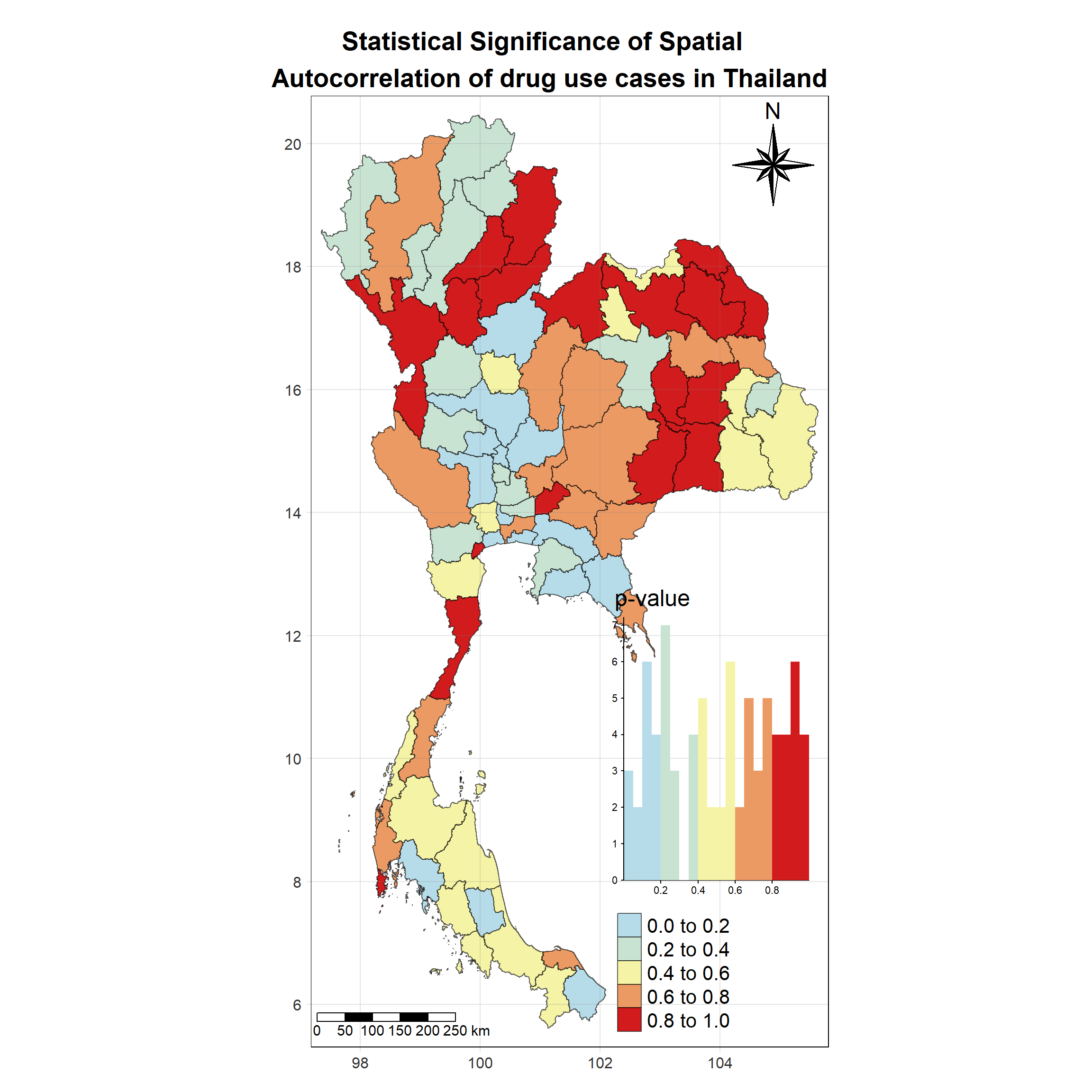

Visualising Statistically Significant Local Spatial Autocorrelation Map

lisa_2020_sig <- lisa_2020  %>%
  filter(p_ii_sim < 0.05) %>% mutate(label = province_en)

tm_shape(lisa_2020)+
  tm_polygons() +
  tm_borders(col = "black", alpha = 0.6)+
tm_shape(lisa_2020_sig)+
  tm_fill("ii", 
          palette = c("#b7dce9","#e1ecbb","#f5f3a6",
                      "#f8d887","#ec9a64","#d21b1c"),
          breaks = c(0, 0.001, 0.01, 0.05, 1),
          labels = c("0.001", "0.01", "0.05", "Not sig"),
          title = "Local Moran's I (p < 0.05)",
          midpoint = NA,
          legend.hist = TRUE, 
          legend.is.portrait = TRUE,
          legend.hist.z = 0.1) +
  tm_borders(col = "black", alpha = 0.6)+
  tm_layout(main.title = "Statistically Significant Village-Level Spatial \n Autocorrelation Map of drug use cases \n in Thailand",
            main.title.position = "center",
            main.title.size = 1.7,
            main.title.fontface = "bold",
            legend.title.size = 1.8,
            legend.text.size = 1.3,
            frame = TRUE) +
  tm_borders(alpha = 0.5) +
  tm_compass(type="8star", text.size = 1.5, size = 3, position=c("RIGHT", "TOP")) +
  tm_scale_bar(position=c("LEFT", "BOTTOM"), text.size=1.2) +
  tm_grid(labels.size = 1,alpha =0.2)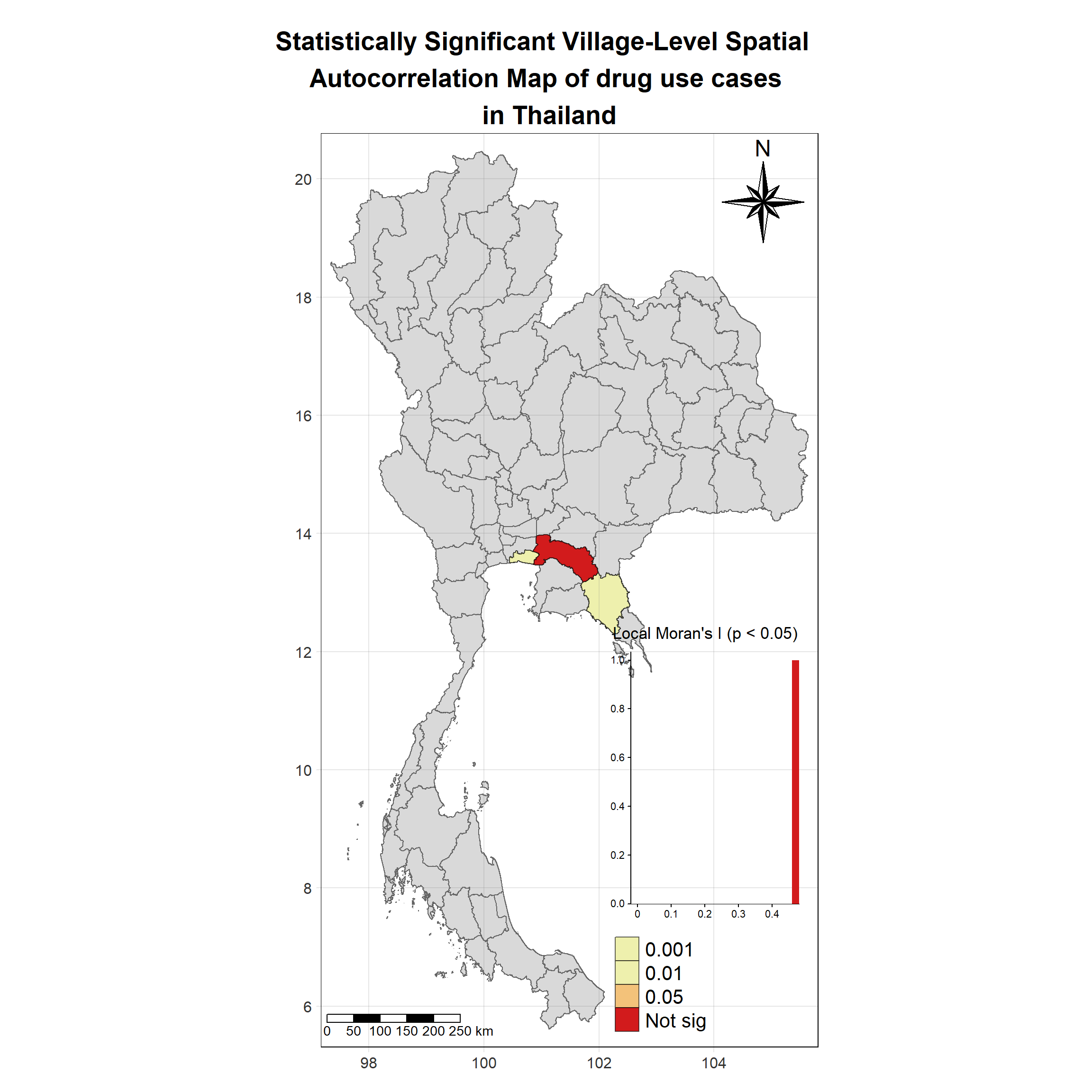

Year 2021

set.seed(4242)
lisa_2021 <- wm_q_2021 %>% 
  mutate(local_moran = local_moran(
    no_cases, nb, wt, nsim = 99),
         .before = 1) %>%
  unnest(local_moran)
lisa_2021

Simple feature collection with 77 features and 21 fields
Geometry type: MULTIPOLYGON
Dimension:     XY
Bounding box:  xmin: 97.34336 ymin: 5.613038 xmax: 105.637 ymax: 20.46507
Geodetic CRS:  WGS 84
# A tibble: 77 × 22
        ii      eii  var_ii   z_ii   p_ii p_ii_sim p_folded_sim skewness
     <dbl>    <dbl>   <dbl>  <dbl>  <dbl>    <dbl>        <dbl>    <dbl>
 1  0.792   0.0225  0.159    1.93  0.0535     0.02         0.01   -0.447
 2  0.0221 -0.00327 0.00190  0.581 0.561      0.6          0.3     0.601
 3 -0.150   0.0186  0.0389  -0.858 0.391      0.38         0.19   -0.813
 4  0.294   0.0143  0.0412   1.38  0.169      0.06         0.03   -0.960
 5  0.118   0.0250  0.0245   0.594 0.553      0.6          0.3    -0.651
 6 -0.321  -0.0164  0.0243  -1.96  0.0501     0.14         0.07   -0.681
 7  0.0681 -0.0366  0.131    0.289 0.773      0.82         0.41   -0.675
 8  0.718   0.0329  0.191    1.57  0.117      0.06         0.03   -0.554
 9  0.635  -0.0222  0.276    1.25  0.211      0.18         0.09   -0.582
10 -0.125  -0.00554 0.0230  -0.790 0.429      0.36         0.18   -0.886
# ℹ 67 more rows
# ℹ 14 more variables: kurtosis <dbl>, mean <fct>, median <fct>, pysal <fct>,
#   nb <nb>, wt <list>, fiscal_year <int>, types_of_drug_offenses <chr>,
#   no_cases <int>, province_en <chr>, Shape_Leng <dbl>, Shape_Area <dbl>,
#   date <date>, geometry <MULTIPOLYGON [°]>

Visualising Local Moran’s I_i

tm_shape(lisa_2021)+
  tm_fill("ii", 
          palette = c("#b7dce9","#e1ecbb","#f5f3a6",
                      "#f8d887","#ec9a64","#d21b1c"),
          title = "Local Moran's I",
          midpoint = NA,
          legend.hist = TRUE, 
          legend.is.portrait = TRUE,
          legend.hist.z = 0.1) +
  tm_borders(col = "black", alpha = 0.6)+
  tm_layout(main.title = "Province-level Spatial Autocorrelation \n of drug use cases in Thailand",
            main.title.position = "center",
            main.title.size = 1.7,
            main.title.fontface = "bold",
            legend.title.size = 1.8,
            legend.text.size = 1.3,
            frame = TRUE) +
  tm_borders(alpha = 0.5) +
  tm_compass(type="8star", text.size = 1.5, size = 3, position=c("RIGHT", "TOP")) +
  tm_scale_bar(position=c("LEFT", "BOTTOM"), text.size=1.2) +
  tm_grid(labels.size = 1,alpha =0.2)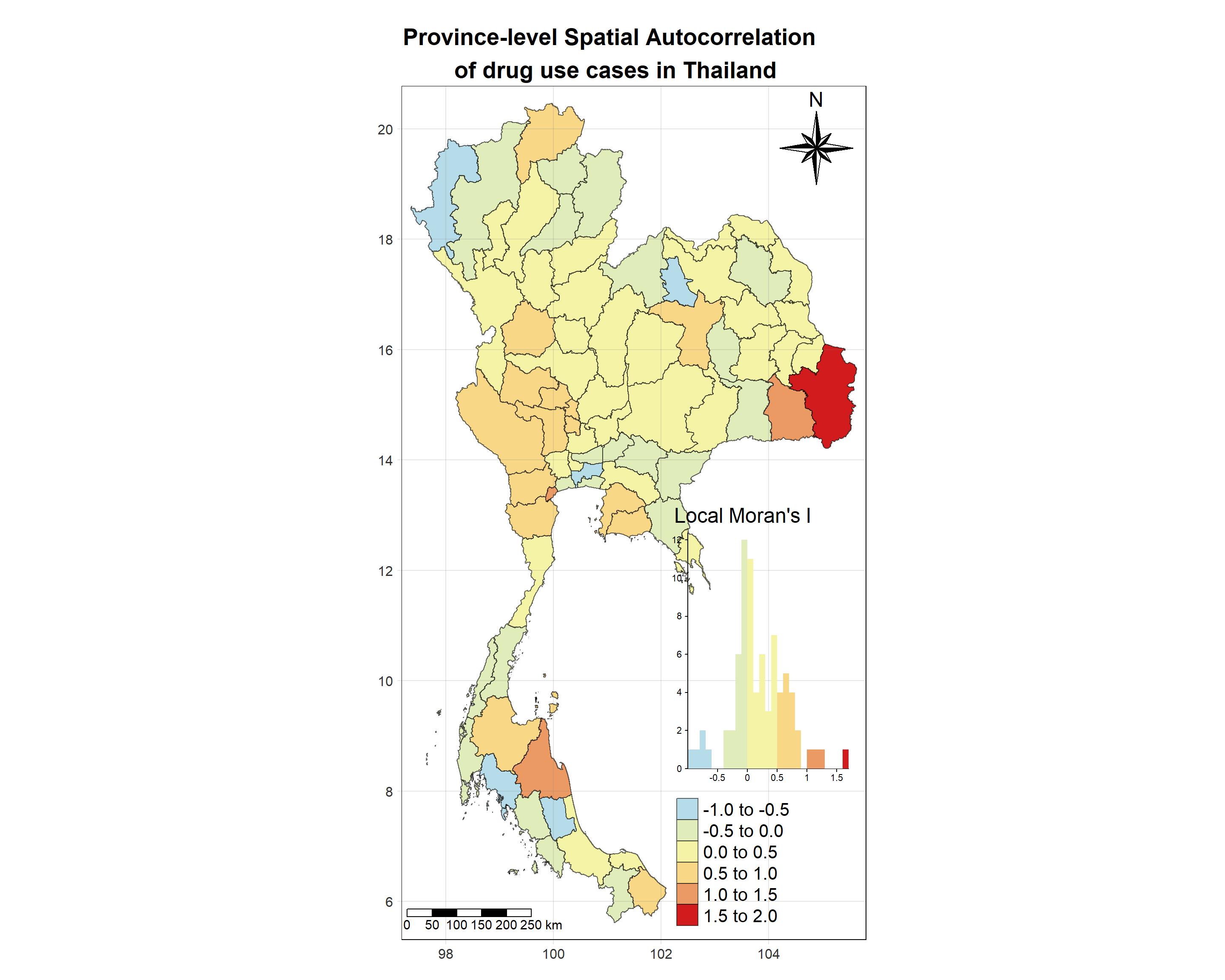

Visualising Local Moran’s I_i p-value

tm_shape(lisa_2021)+
  tm_fill("p_ii_sim", 
          palette = c("#b7dce9","#c9e3d2","#f5f3a6","#ec9a64","#d21b1c"),
          title = "p-value",
          midpoint = NA,
          legend.hist = TRUE, 
          legend.is.portrait = TRUE,
          legend.hist.z = 0.1) +
  tm_borders(col = "black", alpha = 0.6)+
  tm_layout(main.title = "Statistical Significance of Spatial \n Autocorrelation of drug use cases in Thailand",
            main.title.position = "center",
            main.title.size = 1.7,
            main.title.fontface = "bold",
            legend.title.size = 1.8,
            legend.text.size = 1.3,
            frame = TRUE) +
  tm_borders(alpha = 0.5) +
  tm_compass(type="8star", text.size = 1.5, size = 3, position=c("RIGHT", "TOP")) +
  tm_scale_bar(position=c("LEFT", "BOTTOM"), text.size=1.2) +
  tm_grid(labels.size = 1,alpha =0.2)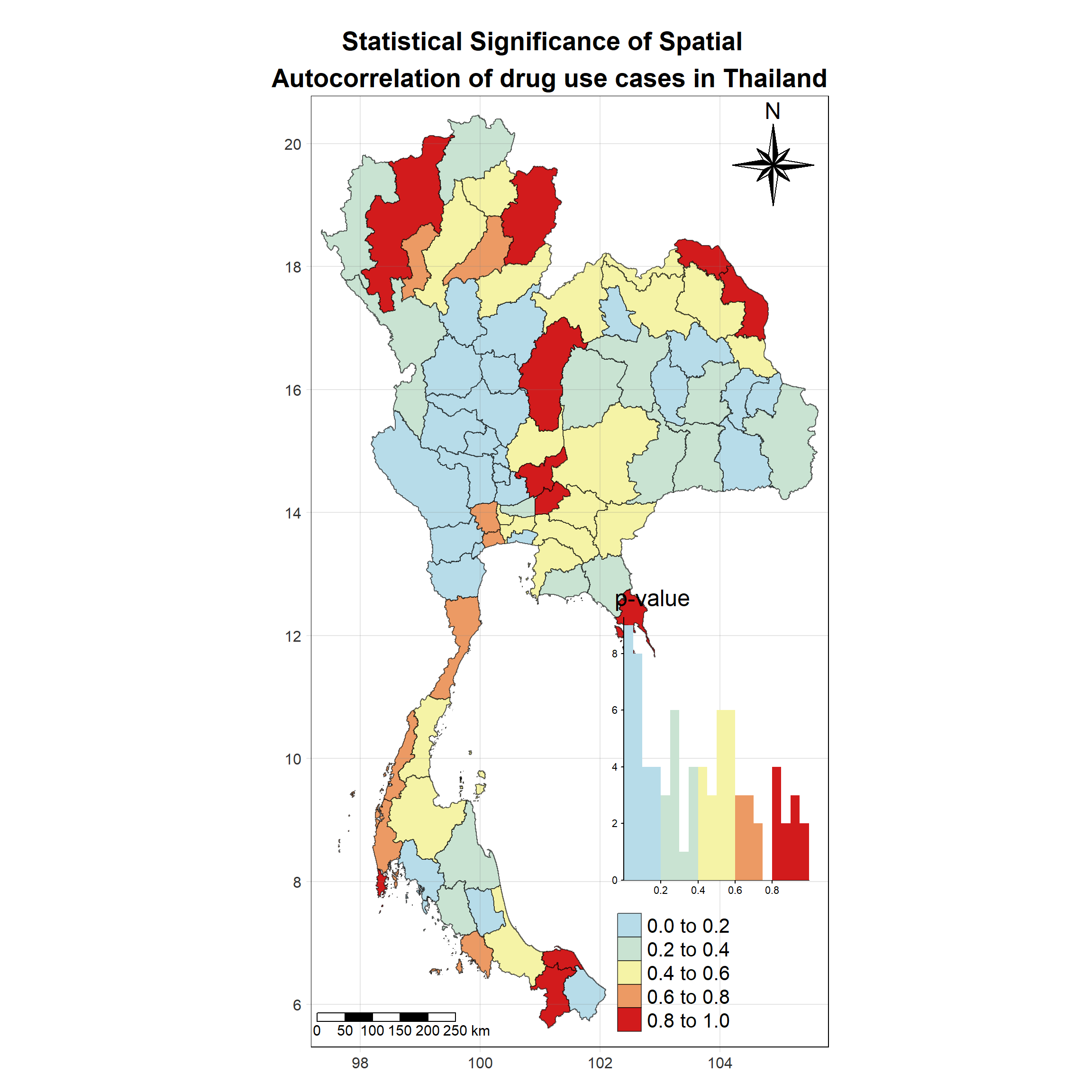

Visualising Statistically Significant Local Spatial Autocorrelation Map

lisa_2021_sig <- lisa_2021  %>%
  filter(p_ii_sim < 0.05) %>% mutate(label = province_en)

tm_shape(lisa_2021)+
  tm_polygons() +
  tm_borders(col = "black", alpha = 0.6)+
tm_shape(lisa_2021_sig)+
  tm_fill("ii", 
          palette = c("#b7dce9","#e1ecbb","#f5f3a6",
                      "#f8d887","#ec9a64","#d21b1c"),
          breaks = c(0, 0.001, 0.01, 0.05, 1),
          labels = c("0.001", "0.01", "0.05", "Not sig"),
          title = "Local Moran's I (p < 0.05)",
          midpoint = NA,
          legend.hist = TRUE, 
          legend.is.portrait = TRUE,
          legend.hist.z = 0.1) +
  tm_borders(col = "black", alpha = 0.6)+
  tm_layout(main.title = "Statistically Significant Village-Level Spatial \n Autocorrelation Map of drug use cases \n in Thailand",
            main.title.position = "center",
            main.title.size = 1.7,
            main.title.fontface = "bold",
            legend.title.size = 1.8,
            legend.text.size = 1.3,
            frame = TRUE) +
  tm_borders(alpha = 0.5) +
  tm_compass(type="8star", text.size = 1.5, size = 3, position=c("RIGHT", "TOP")) +
  tm_scale_bar(position=c("LEFT", "BOTTOM"), text.size=1.2) +
  tm_grid(labels.size = 1,alpha =0.2)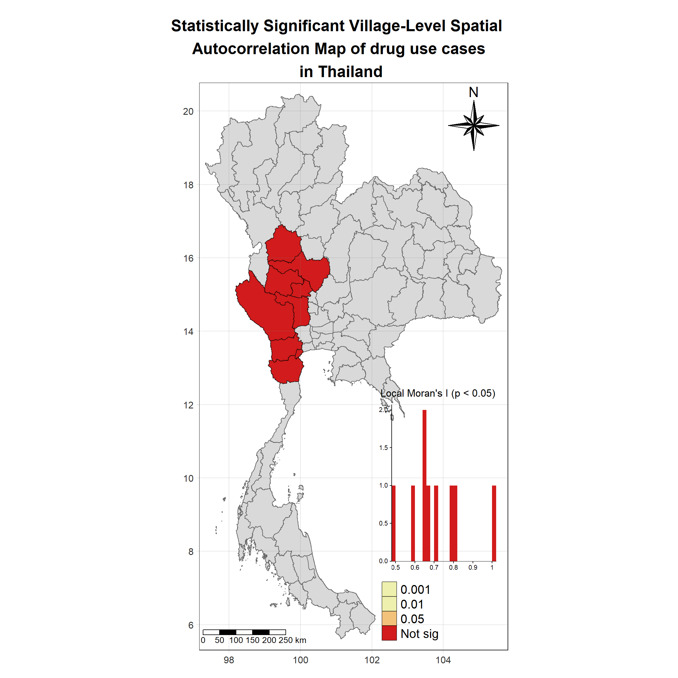

Year 2022

lisa_2022 <- wm_q_2022 %>% 
  mutate(local_moran = local_moran(
    no_cases, nb, wt, nsim = 99),
         .before = 1) %>%
  unnest(local_moran)
lisa_2022

Simple feature collection with 77 features and 21 fields
Geometry type: MULTIPOLYGON
Dimension:     XY
Bounding box:  xmin: 97.34336 ymin: 5.613038 xmax: 105.637 ymax: 20.46507
Geodetic CRS:  WGS 84
# A tibble: 77 × 22
         ii      eii  var_ii    z_ii    p_ii p_ii_sim p_folded_sim skewness
      <dbl>    <dbl>   <dbl>   <dbl>   <dbl>    <dbl>        <dbl>    <dbl>
 1 -0.495    0.0371  0.364   -0.882  0.378       0.36         0.18   -0.139
 2 -0.285    0.0270  0.169   -0.758  0.449       0.46         0.23    0.419
 3  0.0512   0.00125 0.00556  0.670  0.503       0.56         0.28   -0.435
 4  2.11    -0.00674 0.596    2.75   0.00605     0.02         0.01    0.336
 5  0.860    0.0412  0.142    2.17   0.0300      0.02         0.01   -0.661
 6  1.43    -0.0541  0.462    2.18   0.0293      0.04         0.02    0.222
 7 -0.00992 -0.0333  0.0286   0.138  0.890       0.88         0.44   -0.144
 8 -0.00621 -0.00279 0.00210 -0.0747 0.940       0.96         0.48   -0.367
 9  0.0762   0.0177  0.402    0.0922 0.927       0.98         0.49    0.327
10  0.672    0.0326  0.207    1.41   0.159       0.16         0.08   -0.388
# ℹ 67 more rows
# ℹ 14 more variables: kurtosis <dbl>, mean <fct>, median <fct>, pysal <fct>,
#   nb <nb>, wt <list>, fiscal_year <int>, types_of_drug_offenses <chr>,
#   no_cases <int>, province_en <chr>, Shape_Leng <dbl>, Shape_Area <dbl>,
#   date <date>, geometry <MULTIPOLYGON [°]>

Visualising Local Moran’s I_i

tm_shape(lisa_2022)+
  tm_fill("ii", 
          palette = c("#b7dce9","#e1ecbb","#f5f3a6",
                      "#f8d887","#ec9a64","#d21b1c"),
          title = "Local Moran's I",
          midpoint = NA,
          legend.hist = TRUE, 
          legend.is.portrait = TRUE,
          legend.hist.z = 0.1) +
  tm_borders(col = "black", alpha = 0.6)+
  tm_layout(main.title = "Province-level Spatial Autocorrelation \n of drug use cases in Thailand",
            main.title.position = "center",
            main.title.size = 1.7,
            main.title.fontface = "bold",
            legend.title.size = 1.8,
            legend.text.size = 1.3,
            frame = TRUE) +
  tm_borders(alpha = 0.5) +
  tm_compass(type="8star", text.size = 1.5, size = 3, position=c("RIGHT", "TOP")) +
  tm_scale_bar(position=c("LEFT", "BOTTOM"), text.size=1.2) +
  tm_grid(labels.size = 1,alpha =0.2)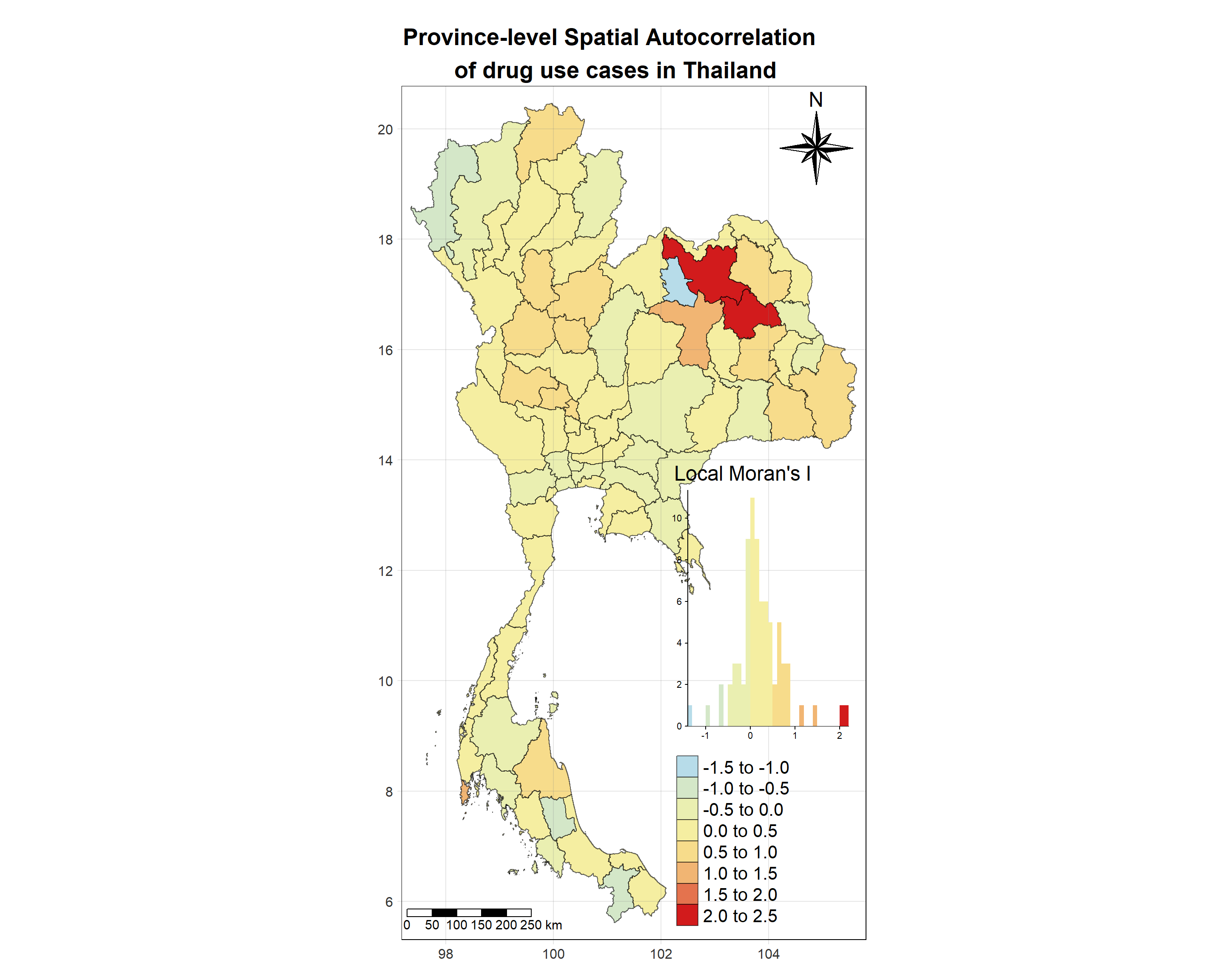

Visualising Local Moran’s I_i p-value

tm_shape(lisa_2022)+
  tm_fill("p_ii_sim", 
          palette = c("#b7dce9","#c9e3d2","#f5f3a6","#ec9a64","#d21b1c"),
          title = "p-value",
          midpoint = NA,
          legend.hist = TRUE, 
          legend.is.portrait = TRUE,
          legend.hist.z = 0.1) +
  tm_borders(col = "black", alpha = 0.6)+
  tm_layout(main.title = "Statistical Significance of Spatial \n Autocorrelation of drug use cases in Thailand",
            main.title.position = "center",
            main.title.size = 1.7,
            main.title.fontface = "bold",
            legend.title.size = 1.8,
            legend.text.size = 1.3,
            frame = TRUE) +
  tm_borders(alpha = 0.5) +
  tm_compass(type="8star", text.size = 1.5, size = 3, position=c("RIGHT", "TOP")) +
  tm_scale_bar(position=c("LEFT", "BOTTOM"), text.size=1.2) +
  tm_grid(labels.size = 1,alpha =0.2)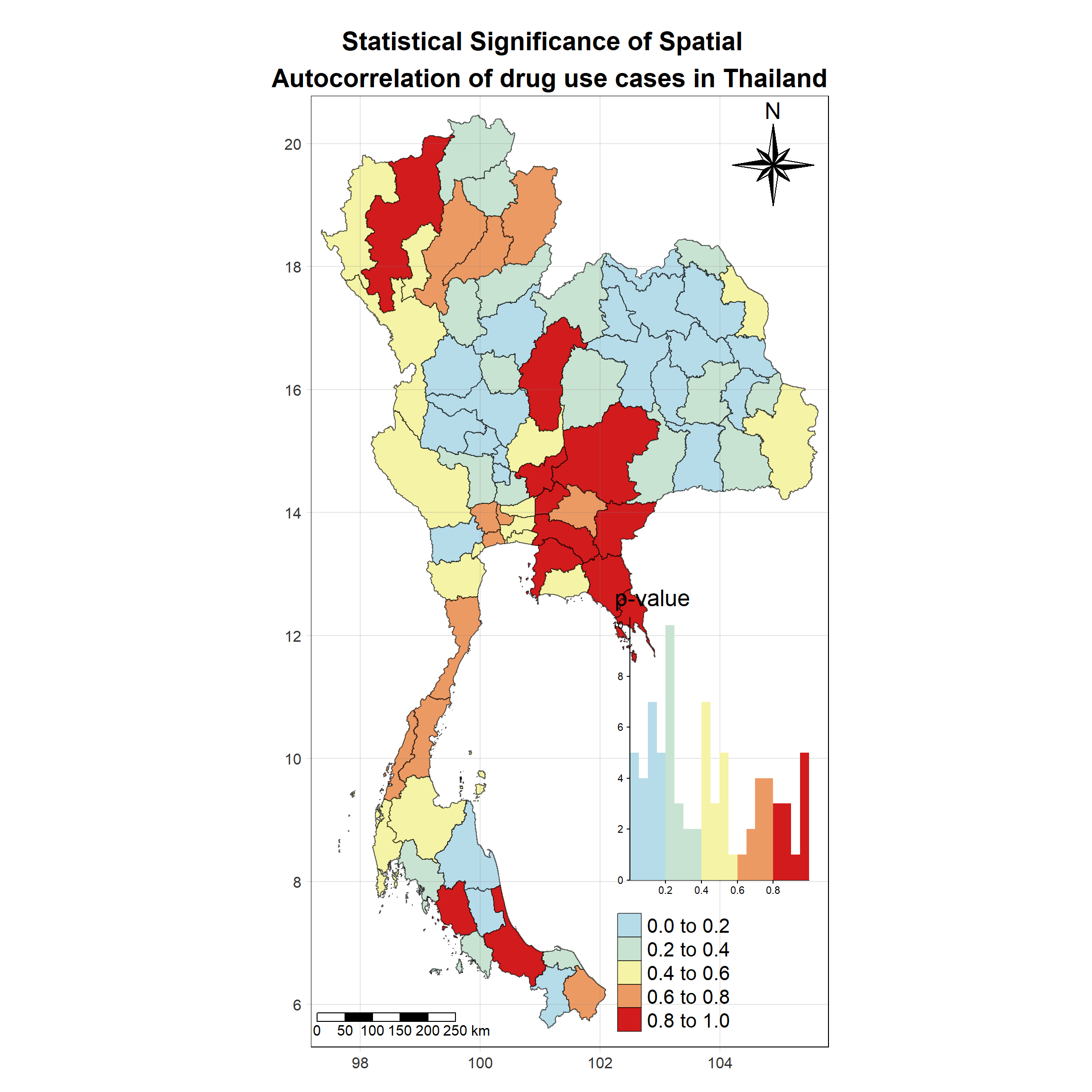

Visualising Statistically Significant Local Spatial Autocorrelation Map

lisa_2022_sig <- lisa_2022  %>%
  filter(p_ii_sim < 0.05) %>% mutate(label = province_en)

tm_shape(lisa_2022)+
  tm_polygons() +
  tm_borders(col = "black", alpha = 0.6)+
tm_shape(lisa_2022_sig)+
  tm_fill("ii", 
          palette = c("#b7dce9","#e1ecbb","#f5f3a6",
                      "#f8d887","#ec9a64","#d21b1c"),
          breaks = c(0, 0.001, 0.01, 0.05, 1),
          labels = c("0.001", "0.01", "0.05", "Not sig"),
          title = "Local Moran's I (p < 0.05)",
          midpoint = NA,
          legend.hist = TRUE, 
          legend.is.portrait = TRUE,
          legend.hist.z = 0.1) +
  tm_borders(col = "black", alpha = 0.6)+
  tm_layout(main.title = "Statistically Significant Village-Level Spatial \n Autocorrelation Map of drug use cases \n in Thailand",
            main.title.position = "center",
            main.title.size = 1.7,
            main.title.fontface = "bold",
            legend.title.size = 1.8,
            legend.text.size = 1.3,
            frame = TRUE) +
  tm_borders(alpha = 0.5) +
  tm_compass(type="8star", text.size = 1.5, size = 3, position=c("RIGHT", "TOP")) +
  tm_scale_bar(position=c("LEFT", "BOTTOM"), text.size=1.2) +
  tm_grid(labels.size = 1,alpha =0.2)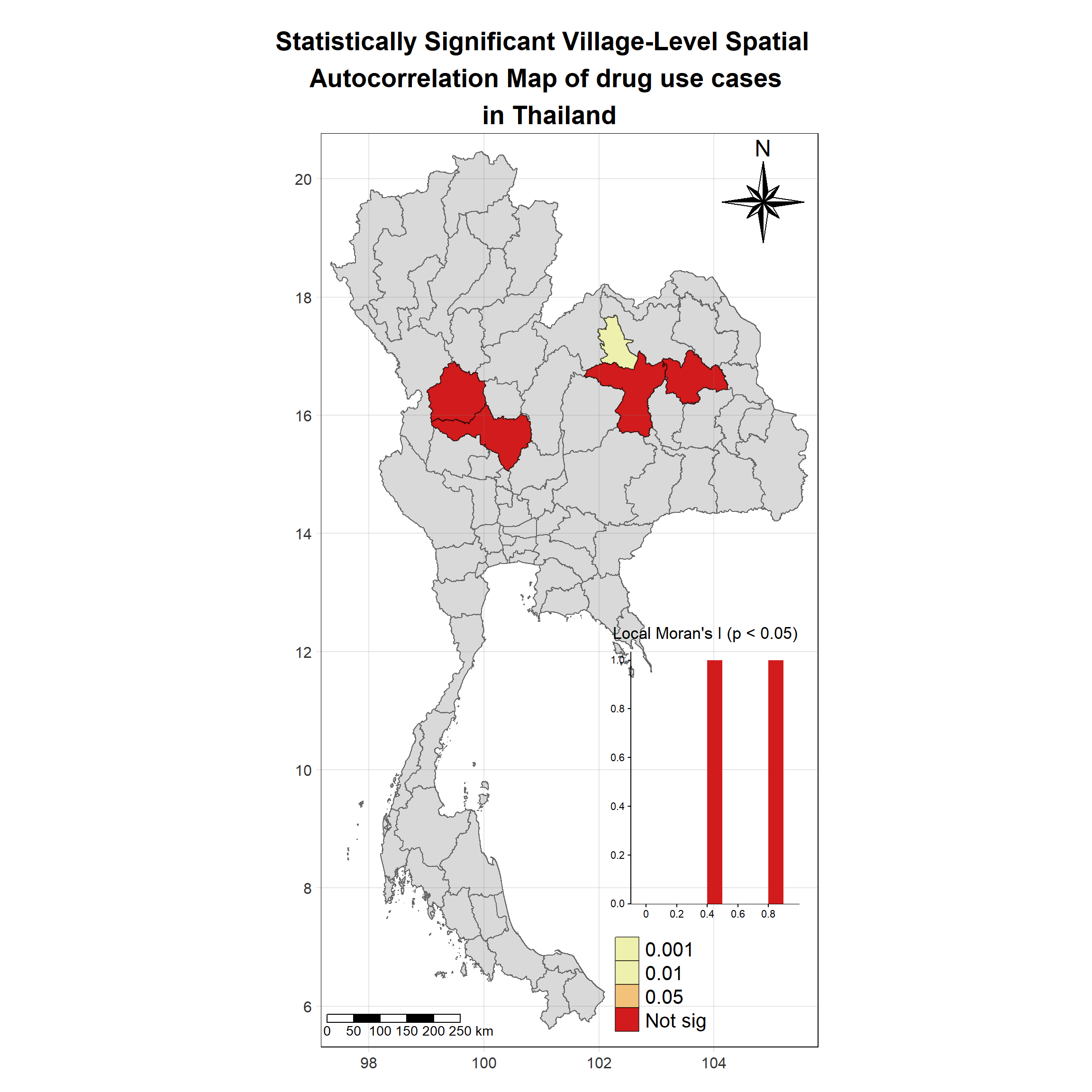

2.7.2 Statistically Significant Local Spatial Autocorrelation Map (2017 - 2022)

We now try to get a detailed view of spatial clusters and outliers in drug use cases across Thailand over a six-year period (2017 - 2022). These maps use Local Moran’s I to detect localized spatial patterns of drug use incidents, identifying regions where there is a statistically significant concentration of high or low case counts compared to neighboring provinces. Each year, the statistically significant clusters (p < 0.05) are highlighted using a color-coded palette that distinguishes between hotspots (areas with high case counts surrounded by similarly high values) and cold spots (areas with low case counts surrounded by low values). By focusing on these spatial patterns, the maps help to uncover specific provinces that either contribute to or deviate from the broader regional trends.

Ultimately, this yearly comparisons aims to allow researchers and policymakers to observe how the spatial distribution of drug-related incidents changes over time. The maps serve as a critical tool for identifying regions where drug use clusters persist or evolve, offering insights into areas that may require targeted interventions. By visualizing the significant local spatial autocorrelation for each year, these maps reveal temporal dynamics, enabling a deeper understanding of the spatial heterogeneity in drug use cases across Thailand.

# List of data for each year
lisa_data <- list(
  "2017" = list(lisa = lisa_2017, sig = lisa_2017_sig),
  "2018" = list(lisa = lisa_2018, sig = lisa_2018_sig),
  "2019" = list(lisa = lisa_2019, sig = lisa_2019_sig),
  "2020" = list(lisa = lisa_2020, sig = lisa_2020_sig),
  "2021" = list(lisa = lisa_2021, sig = lisa_2021_sig),
  "2022" = list(lisa = lisa_2022, sig = lisa_2022_sig)
)

# Initialize an empty list to store tmap objects
maps <- list()

# Loop through each year's data and create a map
for (year in names(lisa_data)) {
  map <- tm_shape(lisa_data[[year]]$lisa) +
    tm_polygons(id = "label") +
    tm_borders(col = "black", alpha = 0.6) +
  tm_shape(lisa_data[[year]]$sig) +
    tm_fill("ii", 
            palette = c("#b7dce9","#e1ecbb","#f5f3a6",
                        "#f8d887","#ec9a64","#d21b1c"),
            breaks = c(0, 0.001, 0.01, 0.05, 1),
            labels = c("0.001", "0.01", "0.05", "Not sig"),
            title = paste("Local Moran's I", year, "(p < 0.05)"),
            midpoint = NA,
            id = "label") +
    tm_borders(col = "black", alpha = 0.6) +
    # Add title to individual plot
    tm_layout(title = paste("Year", year), title.position = c("center", "top"))
  
  # Store the map in the list
  maps[[year]] <- map
}

# Arrange the maps side by side
tmap_arrange(
  maps$`2017`, maps$`2018`, maps$`2019`,
  maps$`2020`, maps$`2021`, maps$`2022`,
  ncol = 3
)

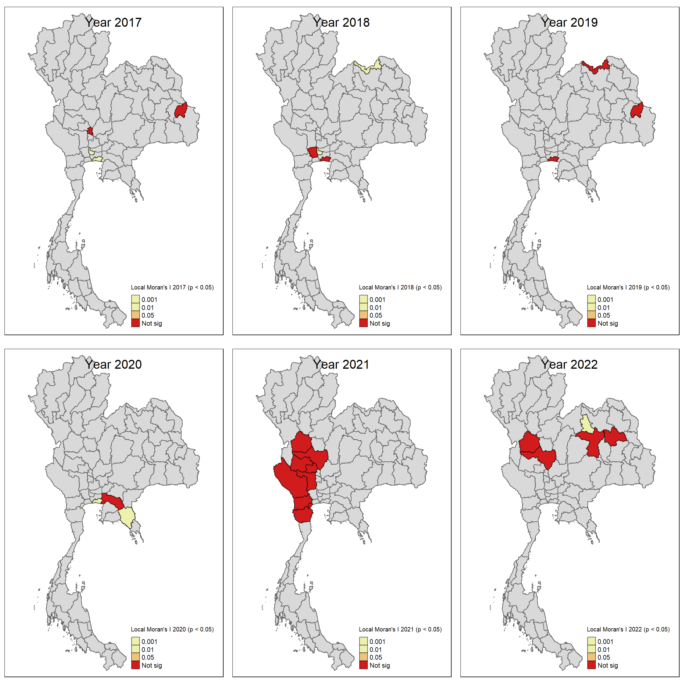
2.7.3 Visualising Statistically Significant Local Spatial Autocorrelation Map

The Local Indicator of Spatial Association (LISA) can provide insights into spatial clustering and outliers of drug-related incidents. Specifically, LISA identifies areas with significant spatial patterns, where the clustering of similar values occurs or where outliers stand out. This can help detect areas with unusually high or low concentrations of drug offenses.

Here’s how we can interpret the LISA classifications for drug use cases:

• High-Low Outliers: Provinces with a high number of drug use cases surrounded by provinces with lower numbers. These could be hotspots of drug activity that differ significantly from their neighbors.

• Low-High Outliers: Provinces with a low number of drug use cases, but surrounded by provinces with higher levels of drug offenses. This could indicate areas with protective factors or lower vulnerability, even though they are located near hotspots.

• High-High Clusters: Provinces with a high concentration of drug use cases, surrounded by provinces that also have high numbers of offenses. This indicates regional hotspots of drug activity where intervention may be needed.

• Low-Low Clusters: Provinces with a low number of drug use cases, surrounded by provinces with similarly low levels. These regions could represent areas with effective prevention measures or lower exposure to drug-related issues.

In each year’s lisa sf data.frame that we created when calculating local Moran’s I, we can find three fields contain the LISA categories. They are mean, median and pysal. We will use mean column to visualise LISA classification maps with relevant tmap functions.

2.7.3.1 Country-wide view

tmap_mode("plot")
study_area_lisa_2017 <- tm_shape(lisa_2017)+
  tm_polygons() +
  tm_borders(col = "black", alpha = 0.6)+
tm_shape(lisa_2017_sig)+
  tm_fill("mean", 
          palette = c("#b7dce9","#ec9a64","#e1ecbb", "#d21b1c"),
          title = "LISA class",
          midpoint = NA,
          legend.hist = TRUE, 
          legend.is.portrait = TRUE,
          legend.hist.z = 0.1) +
  tm_borders(col = "black", alpha = 0.6)+
  tm_layout(main.title = "2017 Thai LISA map",
            main.title.size = 1,
            legend.outside = TRUE,
            legend.outside.position = "right",
            frame = TRUE) +
  tm_borders(alpha = 0.5) +
  tm_scale_bar(position=c("LEFT", "BOTTOM"), text.size=1.2) +
  tm_grid(labels.size = 1,alpha =0.2)

study_area_lisa_2018 <- tm_shape(lisa_2018)+
  tm_polygons() +
  tm_borders(col = "black", alpha = 0.6)+
tm_shape(lisa_2018_sig)+
  tm_fill("mean", 
          palette = c("#b7dce9","#ec9a64","#e1ecbb", "#d21b1c"),
          title = "LISA class",
          midpoint = NA,
          legend.hist = TRUE, 
          legend.is.portrait = TRUE,
          legend.hist.z = 0.1) +
  tm_borders(col = "black", alpha = 0.6)+
  tm_layout(main.title = "2018 Thai LISA map",
            main.title.size = 1,
            legend.outside = TRUE,
            legend.outside.position = "right",
            frame = TRUE) +
  tm_borders(alpha = 0.5) +
  tm_scale_bar(position=c("LEFT", "BOTTOM"), text.size=1.2) +
  tm_grid(labels.size = 1,alpha =0.2)

study_area_lisa_2019 <- tm_shape(lisa_2019)+
  tm_polygons() +
  tm_borders(col = "black", alpha = 0.6)+
tm_shape(lisa_2019_sig)+
  tm_fill("mean", 
          palette = c("#b7dce9","#ec9a64","#e1ecbb", "#d21b1c"),
          title = "LISA class",
          midpoint = NA,
          legend.hist = TRUE, 
          legend.is.portrait = TRUE,
          legend.hist.z = 0.1) +
  tm_borders(col = "black", alpha = 0.6)+
  tm_layout(main.title = "2019 Thai LISA map",
            main.title.size = 1,
            legend.outside = TRUE,
            legend.outside.position = "right",
            frame = TRUE) +
  tm_borders(alpha = 0.5) +
  tm_scale_bar(position=c("LEFT", "BOTTOM"), text.size=1.2) +
  tm_grid(labels.size = 1,alpha =0.2)

study_area_lisa_2020 <- tm_shape(lisa_2020)+
  tm_polygons() +
  tm_borders(col = "black", alpha = 0.6)+
tm_shape(lisa_2020_sig)+
  tm_fill("mean", 
          palette = c("#b7dce9","#ec9a64","#e1ecbb", "#d21b1c"),
          title = "LISA class",
          midpoint = NA,
          legend.hist = TRUE, 
          legend.is.portrait = TRUE,
          legend.hist.z = 0.1) +
  tm_borders(col = "black", alpha = 0.6)+
  tm_layout(main.title = "2020 Thai LISA map",
            main.title.size = 1,
            legend.outside = TRUE,
            legend.outside.position = "right",
            frame = TRUE) +
  tm_borders(alpha = 0.5) +
  tm_scale_bar(position=c("LEFT", "BOTTOM"), text.size=1.2) +
  tm_grid(labels.size = 1,alpha =0.2)

study_area_lisa_2021 <- tm_shape(lisa_2021)+
  tm_polygons() +
  tm_borders(col = "black", alpha = 0.6)+
tm_shape(lisa_2021_sig)+
  tm_fill("mean", 
          palette = c("#b7dce9","#ec9a64","#e1ecbb", "#d21b1c"),
          title = "LISA class",
          midpoint = NA,
          legend.hist = TRUE, 
          legend.is.portrait = TRUE,
          legend.hist.z = 0.1) +
  tm_borders(col = "black", alpha = 0.6)+
  tm_layout(main.title = "2021 Thai LISA map",
            main.title.size = 1,
            legend.outside = TRUE,
            legend.outside.position = "right",
            frame = TRUE) +
  tm_borders(alpha = 0.5) +
  tm_scale_bar(position=c("LEFT", "BOTTOM"), text.size=1.2) +
  tm_grid(labels.size = 1,alpha =0.2)

study_area_lisa_2022 <- tm_shape(lisa_2022)+
  tm_polygons() +
  tm_borders(col = "black", alpha = 0.6)+
tm_shape(lisa_2022_sig)+
  tm_fill("mean", 
          palette = c("#b7dce9","#ec9a64","#e1ecbb", "#d21b1c"),
          title = "LISA class",
          midpoint = NA,
          legend.hist = TRUE, 
          legend.is.portrait = TRUE,
          legend.hist.z = 0.1) +
  tm_borders(col = "black", alpha = 0.6)+
  tm_layout(main.title = "2022 Thai LISA map",
            main.title.size = 1,
            legend.outside = TRUE,
            legend.outside.position = "right",
            frame = TRUE) +
  tm_borders(alpha = 0.5) +
  tm_scale_bar(position=c("LEFT", "BOTTOM"), text.size=1.2) +
  tm_grid(labels.size = 1,alpha =0.2)

Year 2017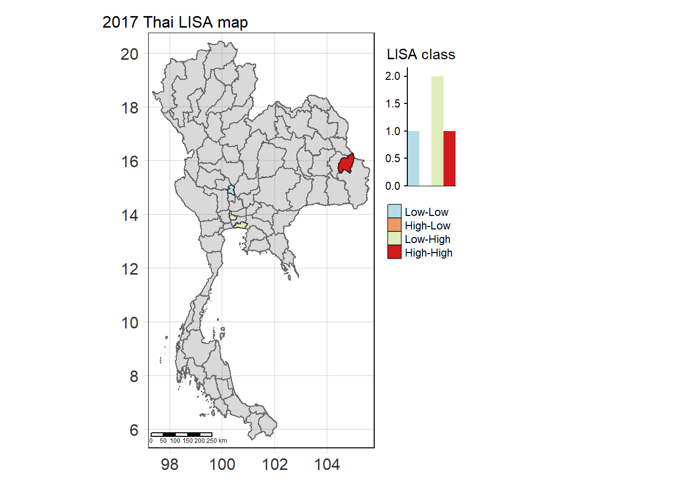

study_area_lisa_2017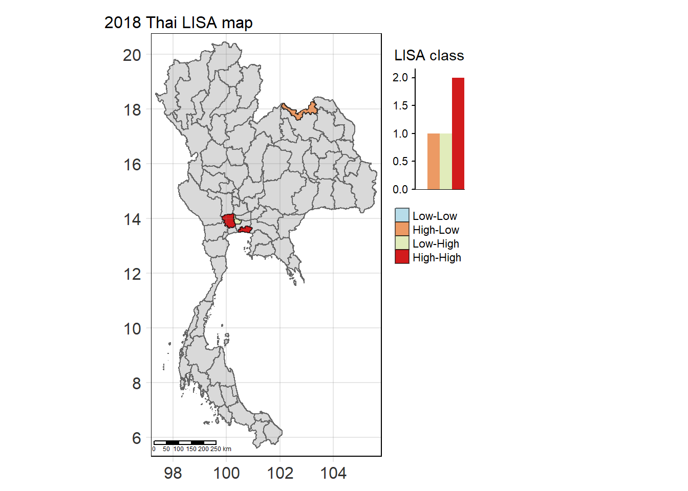

Year 2018

study_area_lisa_2018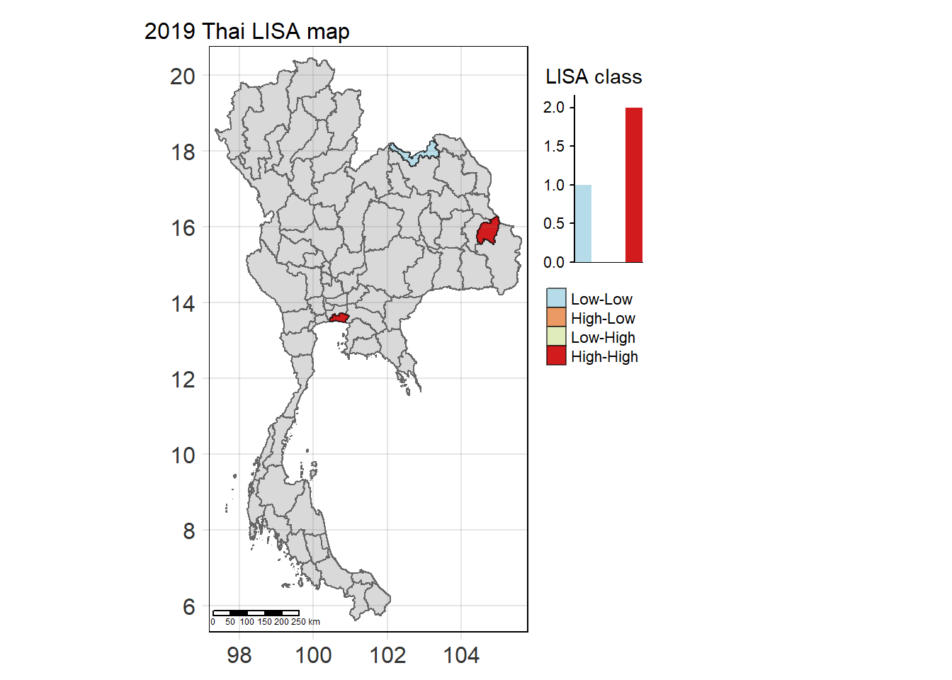

Year 2019

study_area_lisa_2019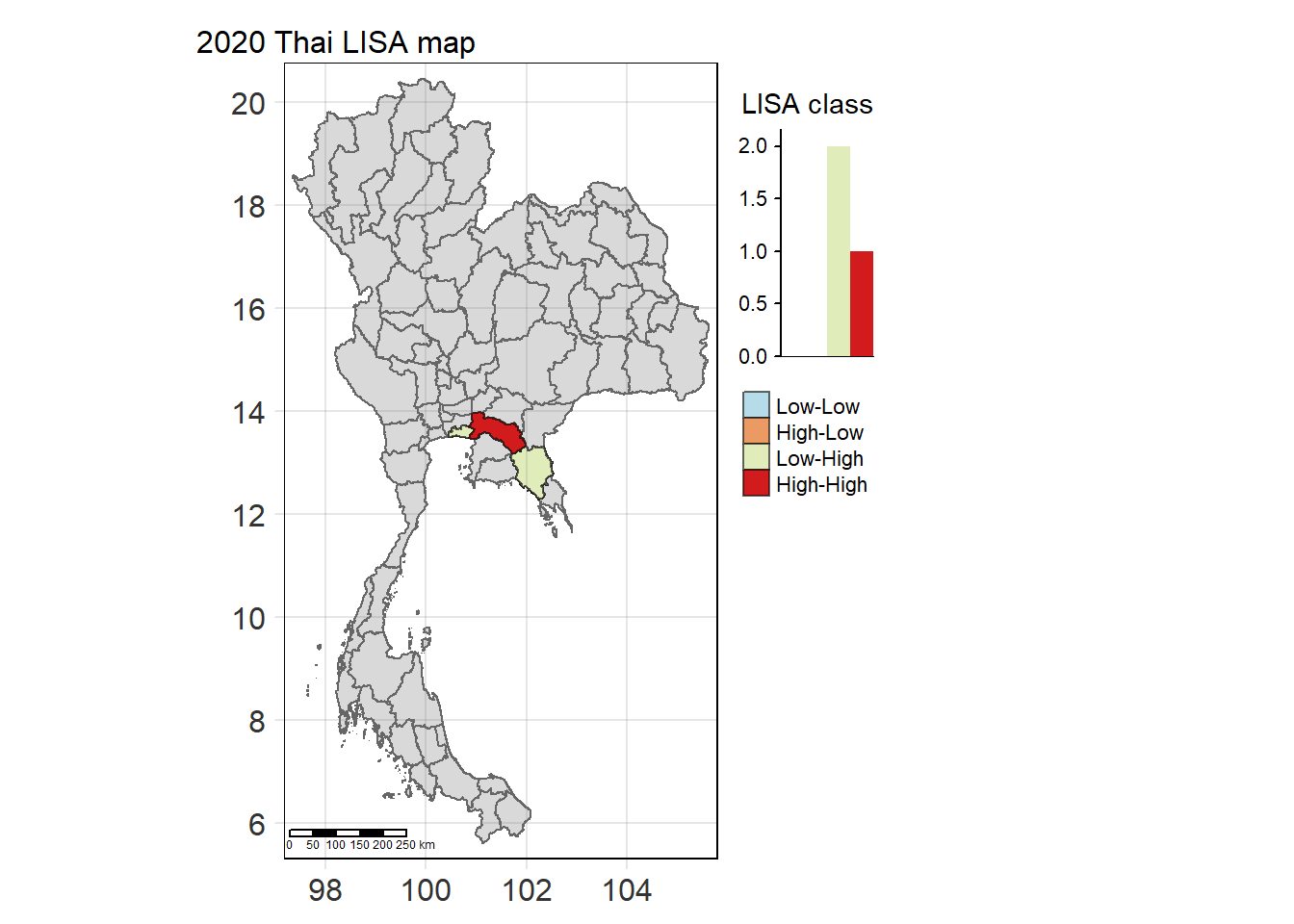

Year 2020

study_area_lisa_2020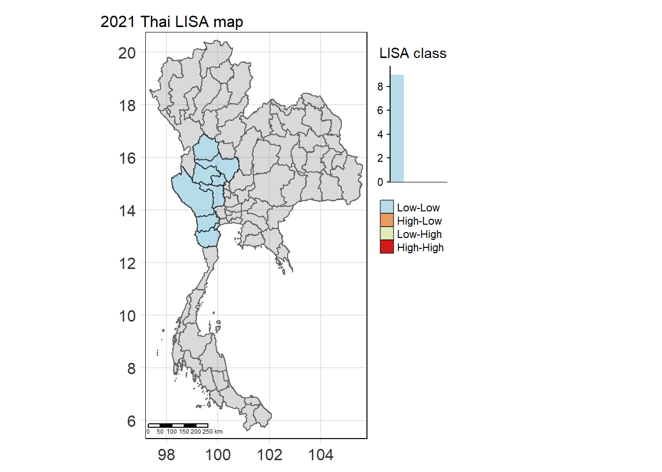

Year 2021

study_area_lisa_2021

Year 2022

study_area_lisa_2022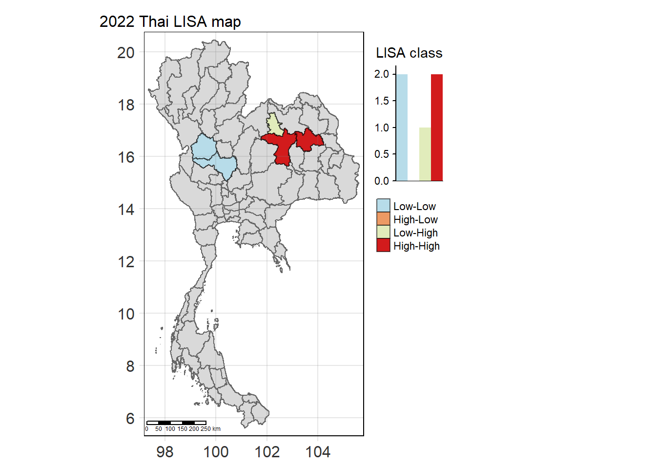

On a national scale, provinces, especially smaller ones, may appear too small to analyze effectively, making it difficult to clearly see the distribution of the LISA classifications. A regional view, with better zoom and focus, can improve the clarity of visualization. It becomes easier to distinguish between clusters and outliers, especially in densely populated or small-area provinces.

2.7.3.2 Regional view

Thailand is variably divided into different sets of regions, the most notable of which are the six-region grouping used in geographic studies, and the four-region grouping consistent with the Monthon administrative regional grouping system formerly used by the Ministry of Interior. These regions are the largest subdivisions of the country.

In contrast to the administrative divisions of the provinces of Thailand, the regions no longer have an administrative character, but are used for statistical or academic purposes.

A six-region system is commonly used for geographical and scientific purposes. This system dates to 1935. It was formalised in 1977 by the National Geographical Committee, which was appointed by the National Research Council. It divides the country into the following regions:

• Northern Thailand
• Northeastern Thailand
• Western Thailand
• Central Thailand
• Eastern Thailand
• Southern Thailand

The four-region system, used in some administrative and statistical contexts, and also as a loose cultural grouping, includes the western and eastern regions within the central region, while grouping the provinces of Sukhothai, Phitsanulok, Phichit, Kamphaeng Phet, Phetchabun, Nakhon Sawan, and Uthai Thani in the northern region. This is also the regional system most commonly used on national television, when discussing regional events. It divides the country into the following regions:

• Northern Thailand
• Northeastern Thailand (Isan)
• Central Thailand
• Southern Thailand

The Thai Meteorological Department divides the country into six regions for meteorological purposes. It differs from the four-region system in that the east is regarded as a separate region, the south is divided into east and west coasts, and Nakhon Sawan and Uthai Thani are grouped in the central region.

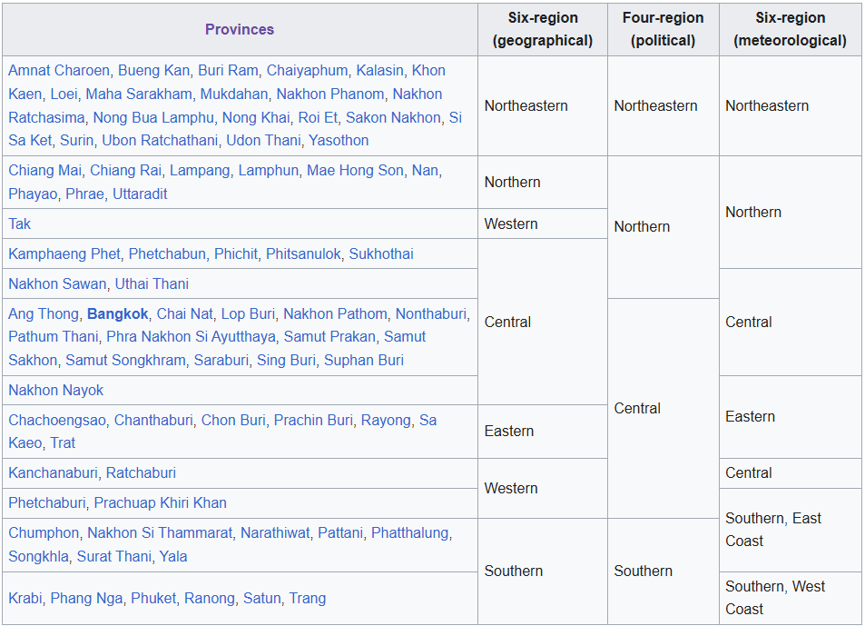
Notes

LISA relies on the spatial relationships between neighboring areas. If you remove certain provinces from the analysis when zooming into a region, the LISA statistics could change due to the loss of spatial context. To maintain the integrity of LISA classifications in a regional view, we will ensure that the entire neighborhood structure is still considered. Even though you may only visualize a specific region, the calculations should still include all neighboring provinces, not just those within the selected region.

It is important to keep the spatial dependencies intact by including all neighboring provinces in the LISA calculations. This ensures that the regional LISA classifications remain consistent with the national analysis, and the spatial clustering or outlier detection is not compromised due to changes in the geographical scope. The regional view should be treated as a zoomed-in perspective of the national LISA results, without altering the underlying spatial relationships.

Given the geographical scope of the study, we will adopt a six-region geographical distribution, focusing on the provincial level. This approach not only allows for a regionally nuanced analysis but also reduces the computational load within the R environment, making the analysis more efficient.

# Define provinces for each region
northeastern <- c("Amnat Charoen", "Bueng Kan", "Buri Ram", "Chaiyaphum", "Kalasin", 
                  "Khon Kaen", "Loei", "Maha Sarakham", "Mukdahan", "Nakhon Phanom", 
                  "Nakhon Ratchasima", "Nong Bua Lam Phu", "Nong Khai", "Roi Et", 
                  "Sakon Nakhon", "Si Sa Ket", "Surin", "Ubon Ratchathani", "Udon Thani", 
                  "Yasothon")

northern <- c("Chiang Mai", "Chiang Rai", "Lampang", "Lamphun", "Mae Hong Son", 
              "Nan", "Phayao", "Phrae", "Uttaradit")

western <- c("Tak", "Kanchanaburi", "Ratchaburi", "Phetchaburi", "Prachuap Khiri Khan")

central <- c("Kamphaeng Phet", "Phetchabun", "Phichit", "Phitsanulok", "Sukhothai", 
             "Nakhon Sawan", "Uthai Thani", "Ang Thong", "Bangkok", "Chai Nat", 
             "Lop Buri", "Nakhon Pathom", "Nonthaburi", "Pathum Thani", 
             "Phra Nakhon Si Ayutthaya", "Samut Prakan", "Samut Sakhon", 
             "Samut Songkhram", "Saraburi", "Sing Buri", "Suphan Buri", "Nakhon Nayok")

eastern <- c("Chachoengsao", "Chanthaburi", "Chon Buri", "Prachin Buri", "Rayong", 
             "Sa Kaeo", "Trat")

southern <- c("Chumphon", "Nakhon Si Thammarat", "Narathiwat", "Pattani", 
              "Phatthalung", "Songkhla", "Surat Thani", "Yala", "Krabi", 
              "Phangnga", "Phuket", "Ranong", "Satun", "Trang")

Using a combination of the Local Moran’s I plot, which visualizes the degree of spatial autocorrelation, and the p-value plot, which highlights statistically significant areas, we can gain deeper insights into the spatial dynamics of drug use incidents within the region. This dual visualization approach ensures that identified patterns are both meaningful and reliable, allowing for more informed decision-making in policy development and resource allocation to tackle drug-related issues in specific regions.

Notes

The Local Moran’s I plot and the p-value of Local Moran’s I plot work together to help identify significant spatial patterns in the distribution of drug use cases across regions. The Local Moran’s I plot shows the degree of spatial autocorrelation, indicating where clusters of similar values (either high or low) occur. This plot helps highlight potential hotspots (high values surrounded by high values) or cold spots (low values surrounded by low values), as well as potential outliers (where high values are surrounded by low values or vice versa).

However, the Local Moran’s I values alone do not indicate whether these patterns are statistically significant. This is where the p-value of Local Moran’s I plot comes into play. It shows the significance levels of the spatial patterns, with red areas indicating highly significant clusters and blue/green areas representing non-significant patterns. This plot helps validate whether the clusters or outliers seen in the Local Moran’s I plot are meaningful or if they occurred randomly.

By using both plots together, we can accurately classify regions into LISA categories such as High-High clusters (significant hotspots of high drug use cases), Low-Low clusters (regions of low drug use cases surrounded by similar values), and outliers (provinces where values deviate significantly from their neighbors). The combination of these plots ensures that we can distinguish between true spatial patterns and random variation, leading to more reliable insights into the distribution of drug-related incidents.

Year 2017

northeastern_lisa_2017 <- lisa_2017 %>% filter(province_en %in% northeastern)
northern_lisa_2017 <- lisa_2017 %>% filter(province_en %in% northern)
western_lisa_2017 <- lisa_2017 %>% filter(province_en %in% western)
central_lisa_2017 <- lisa_2017 %>% filter(province_en %in% central)
eastern_lisa_2017 <- lisa_2017 %>% filter(province_en %in% eastern)
southern_lisa_2017 <- lisa_2017 %>% filter(province_en %in% southern)

northeastern_lisa_2017_sig <- lisa_2017_sig %>% filter(province_en %in% northeastern)
northern_lisa_2017_sig <- lisa_2017_sig %>% filter(province_en %in% northern)
western_lisa_2017_sig <- lisa_2017_sig %>% filter(province_en %in% western)
central_lisa_2017_sig <- lisa_2017_sig %>% filter(province_en %in% central)
eastern_lisa_2017_sig <- lisa_2017_sig %>% filter(province_en %in% eastern)
southern_lisa_2017_sig <- lisa_2017_sig %>% filter(province_en %in% southern)

Northeastern Region

northeastern_local <- tm_shape(northeastern_lisa_2017)+
  tm_fill("ii", 
          palette = c("#e1ecbb","#f5f3a6", "#ec9a64","#de573e","#d21b1c"),
          title = "Local Moran's I",
          midpoint = NA) +
  tm_borders(col = "black", alpha = 0.6)+
  tm_layout(main.title = "Village-Level Spatial Autocorrelation \nof drug use cases in Northeastern Region",
            main.title.position = "center",
            main.title.size = 1.3,
            main.title.fontface = "bold",
            legend.title.size = 1,
            legend.text.size = 0.8,
            frame = TRUE) +
  tm_borders(alpha = 0.5) +
  tm_compass(type="8star", text.size = 1, size = 2, position=c("RIGHT", "TOP")) +
  tm_scale_bar(position=c("LEFT", "BOTTOM"), text.size=1) +
  tm_grid(labels.size = 1,alpha =0.2)

northeastern_sig <- tm_shape(northeastern_lisa_2017)+
  tm_fill("p_ii_sim", 
          palette = c("#d21b1c","#ec9a64","#f5f3a6","#c9e3d2","#b7dce9"),
          breaks = c(0, 0.001, 0.01, 0.05, 1),
          labels = c("0.001", "0.01", "0.05", "Not sig"), 
          title = "p-value",
          midpoint = NA) +
  tm_borders(col = "black", alpha = 0.6)+
  tm_layout(main.title = "Statistical Significance of Spatial Autocorrelation\n of drug use cases in Northeastern Region",
            main.title.position = "center",
            main.title.size = 1.3,
            main.title.fontface = "bold",
            legend.title.size = 1,
            legend.text.size = 0.8,
            frame = TRUE) +
  tm_borders(alpha = 0.5) +
  tm_compass(type="8star", text.size = 1, size = 2, position=c("RIGHT", "TOP")) +
  tm_scale_bar(position=c("LEFT", "BOTTOM"), text.size=1) +
  tm_grid(labels.size = 1,alpha =0.2)

tmap_arrange(northeastern_local,northeastern_sig, asp=1, ncol=2)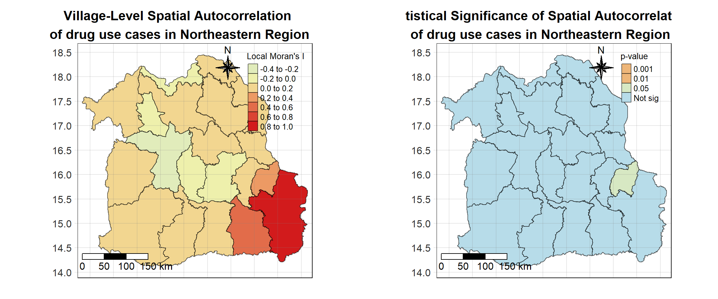

Northern Region

northern_local <- tm_shape(northern_lisa_2017)+
  tm_fill("ii", 
          palette = c("#e1ecbb","#f5f3a6", "#ec9a64","#de573e","#d21b1c"),
          title = "Local Moran's I",
          midpoint = NA) +
  tm_borders(col = "black", alpha = 0.6)+
  tm_layout(main.title = "Village-Level Spatial Autocorrelation \nof drug use cases in Northern Region",
            main.title.position = "center",
            main.title.size = 1.3,
            main.title.fontface = "bold",
            legend.title.size = 1,
            legend.text.size = 0.8,
            frame = TRUE) +
  tm_borders(alpha = 0.5) +
  tm_compass(type="8star", text.size = 1, size = 2, position=c("RIGHT", "TOP")) +
  tm_scale_bar(position=c("LEFT", "BOTTOM"), text.size=1) +
  tm_grid(labels.size = 1,alpha =0.2)

northern_sig <- tm_shape(northern_lisa_2017)+
  tm_fill("p_ii_sim", 
          palette = c("#d21b1c","#ec9a64","#f5f3a6","#c9e3d2","#b7dce9"),
          breaks = c(0, 0.001, 0.01, 0.05, 1),
          labels = c("0.001", "0.01", "0.05", "Not sig"), 
          title = "p-value",
          midpoint = NA) +
  tm_borders(col = "black", alpha = 0.6)+
  tm_layout(main.title = "Statistical Significance of Spatial Autocorrelation\n of drug use cases in Northern Region",
            main.title.position = "center",
            main.title.size = 1.3,
            main.title.fontface = "bold",
            legend.title.size = 1,
            legend.text.size = 0.8,
            frame = TRUE) +
  tm_borders(alpha = 0.5) +
  tm_compass(type="8star", text.size = 1, size = 2, position=c("RIGHT", "TOP")) +
  tm_scale_bar(position=c("LEFT", "BOTTOM"), text.size=1) +
  tm_grid(labels.size = 1,alpha =0.2)

tmap_arrange(northern_local,northern_sig, asp=1, ncol=2)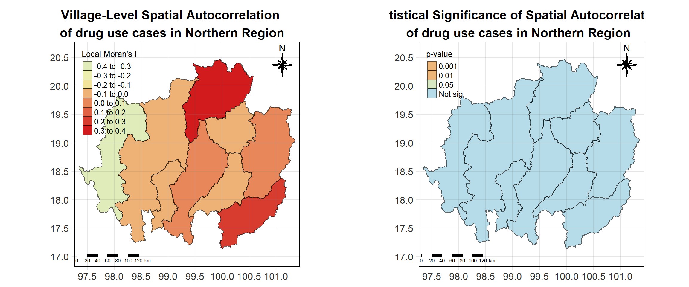

Western Region

western_local <- tm_shape(western_lisa_2017)+
  tm_fill("ii", 
          palette = c("#e1ecbb","#f5f3a6", "#ec9a64","#de573e","#d21b1c"),
          title = "Local Moran's I",
          midpoint = NA) +
  tm_borders(col = "black", alpha = 0.6)+
  tm_layout(main.title = "Village-Level Spatial Autocorrelation \nof drug use cases in Western Region",
            main.title.position = "center",
            main.title.size = 1.3,
            main.title.fontface = "bold",
            legend.title.size = 1,
            legend.text.size = 0.8,
            frame = TRUE) +
  tm_borders(alpha = 0.5) +
  tm_compass(type="8star", text.size = 1, size = 2, position=c("RIGHT", "TOP")) +
  tm_scale_bar(position=c("LEFT", "BOTTOM"), text.size=1) +
  tm_grid(labels.size = 1,alpha =0.2)

western_sig <- tm_shape(western_lisa_2017)+
  tm_fill("p_ii_sim", 
          palette = c("#d21b1c","#ec9a64","#f5f3a6","#c9e3d2","#b7dce9"),
          breaks = c(0, 0.001, 0.01, 0.05, 1),
          labels = c("0.001", "0.01", "0.05", "Not sig"), 
          title = "p-value",
          midpoint = NA) +
  tm_borders(col = "black", alpha = 0.6)+
  tm_layout(main.title = "Statistical Significance of Spatial Autocorrelation\n of drug use cases in Western Region",
            main.title.position = "center",
            main.title.size = 1.3,
            main.title.fontface = "bold",
            legend.title.size = 1,
            legend.text.size = 0.8,
            frame = TRUE) +
  tm_borders(alpha = 0.5) +
  tm_compass(type="8star", text.size = 1, size = 2, position=c("RIGHT", "TOP")) +
  tm_scale_bar(position=c("LEFT", "BOTTOM"), text.size=1) +
  tm_grid(labels.size = 1,alpha =0.2)

tmap_arrange(western_local,western_sig, asp=1, ncol=2)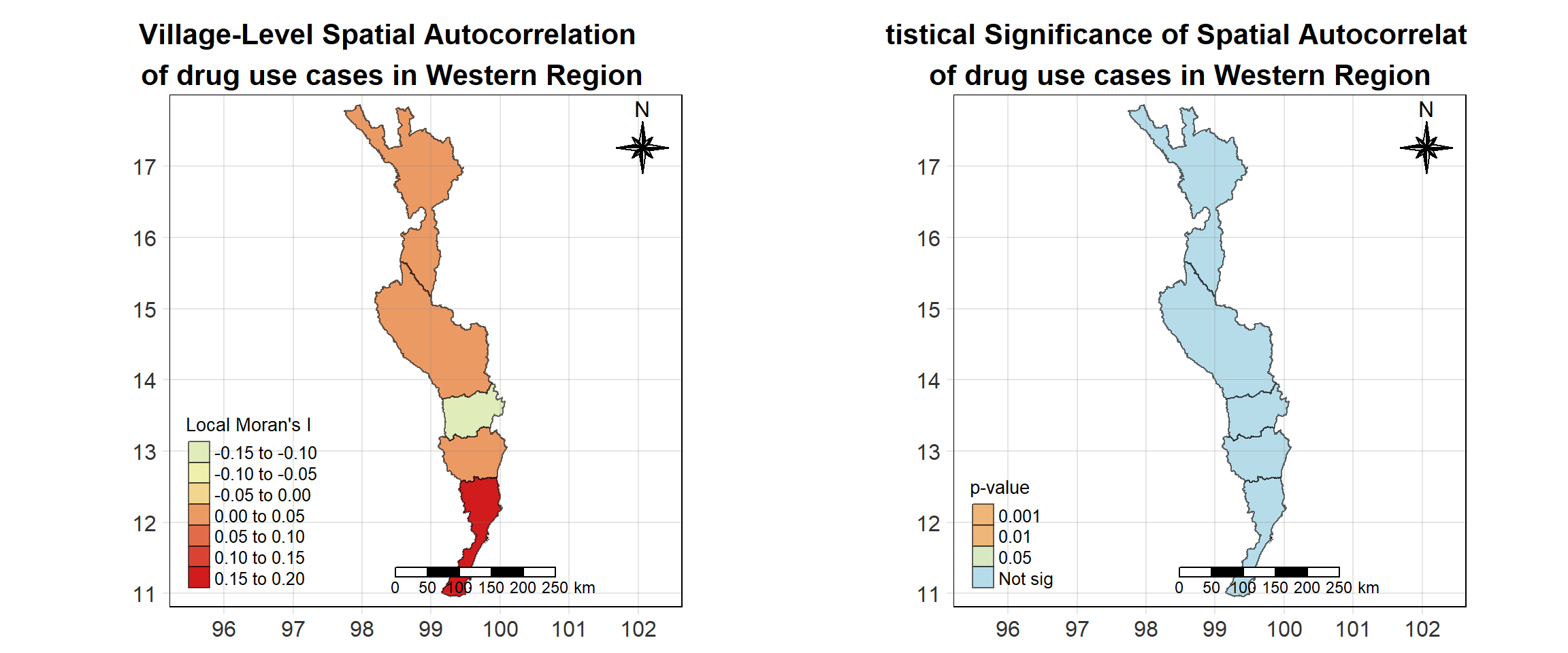

Central Region

central_local <- tm_shape(central_lisa_2017)+
  tm_fill("ii", 
          palette = c("#e1ecbb","#f5f3a6", "#ec9a64","#de573e","#d21b1c"),
          title = "Local Moran's I",
          midpoint = NA) +
  tm_borders(col = "black", alpha = 0.6)+
  tm_layout(main.title = "Village-Level Spatial Autocorrelation \nof drug use cases in Central Region",
            main.title.position = "center",
            main.title.size = 1.3,
            main.title.fontface = "bold",
            legend.title.size = 1,
            legend.text.size = 0.8,
            frame = TRUE) +
  tm_borders(alpha = 0.5) +
  tm_compass(type="8star", text.size = 1, size = 2, position=c("RIGHT", "TOP")) +
  tm_scale_bar(position=c("LEFT", "BOTTOM"), text.size=1) +
  tm_grid(labels.size = 1,alpha =0.2)

central_sig <- tm_shape(central_lisa_2017)+
  tm_fill("p_ii_sim", 
          palette = c("#d21b1c","#ec9a64","#f5f3a6","#c9e3d2","#b7dce9"),
          breaks = c(0, 0.001, 0.01, 0.05, 1),
          labels = c("0.001", "0.01", "0.05", "Not sig"), 
          title = "p-value",
          midpoint = NA) +
  tm_borders(col = "black", alpha = 0.6)+
  tm_layout(main.title = "Statistical Significance of Spatial Autocorrelation\n of drug use cases in Central Region",
            main.title.position = "center",
            main.title.size = 1.3,
            main.title.fontface = "bold",
            legend.title.size = 1,
            legend.text.size = 0.8,
            frame = TRUE) +
  tm_borders(alpha = 0.5) +
  tm_compass(type="8star", text.size = 1, size = 2, position=c("RIGHT", "TOP")) +
  tm_scale_bar(position=c("LEFT", "BOTTOM"), text.size=1) +
  tm_grid(labels.size = 1,alpha =0.2)

tmap_arrange(central_local,central_sig, asp=1, ncol=2)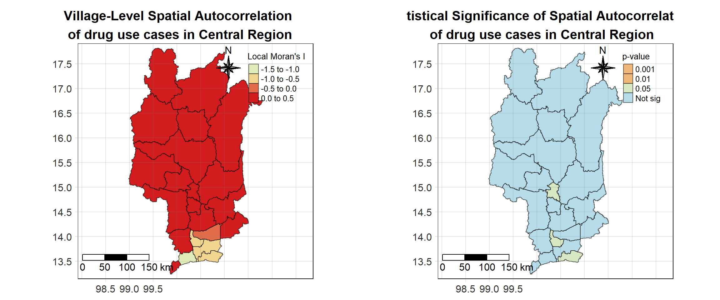

Eastern Region

eastern_local <- tm_shape(eastern_lisa_2017)+
  tm_fill("ii", 
          palette = c("#e1ecbb","#f5f3a6", "#ec9a64","#de573e","#d21b1c"),
          title = "Local Moran's I",
          midpoint = NA) +
  tm_borders(col = "black", alpha = 0.6)+
  tm_layout(main.title = "Village-Level Spatial Autocorrelation \nof drug use cases in Eastern Region",
            main.title.position = "center",
            main.title.size = 1.3,
            main.title.fontface = "bold",
            legend.title.size = 1,
            legend.text.size = 0.8,
            frame = TRUE) +
  tm_borders(alpha = 0.5) +
  tm_compass(type="8star", text.size = 1, size = 2, position=c("RIGHT", "TOP")) +
  tm_scale_bar(position=c("LEFT", "BOTTOM"), text.size=1) +
  tm_grid(labels.size = 1,alpha =0.2)

eastern_sig <- tm_shape(eastern_lisa_2017)+
  tm_fill("p_ii_sim", 
          palette = c("#d21b1c","#ec9a64","#f5f3a6","#c9e3d2","#b7dce9"),
          breaks = c(0, 0.001, 0.01, 0.05, 1),
          labels = c("0.001", "0.01", "0.05", "Not sig"), 
          title = "p-value",
          midpoint = NA) +
  tm_borders(col = "black", alpha = 0.6)+
  tm_layout(main.title = "Statistical Significance of Spatial Autocorrelation\n of drug use cases in Eastern Region",
            main.title.position = "center",
            main.title.size = 1.3,
            main.title.fontface = "bold",
            legend.title.size = 1,
            legend.text.size = 0.8,
            frame = TRUE) +
  tm_borders(alpha = 0.5) +
  tm_compass(type="8star", text.size = 1, size = 2, position=c("RIGHT", "TOP")) +
  tm_scale_bar(position=c("LEFT", "BOTTOM"), text.size=1) +
  tm_grid(labels.size = 1,alpha =0.2)

tmap_arrange(eastern_local,eastern_sig, asp=1, ncol=2)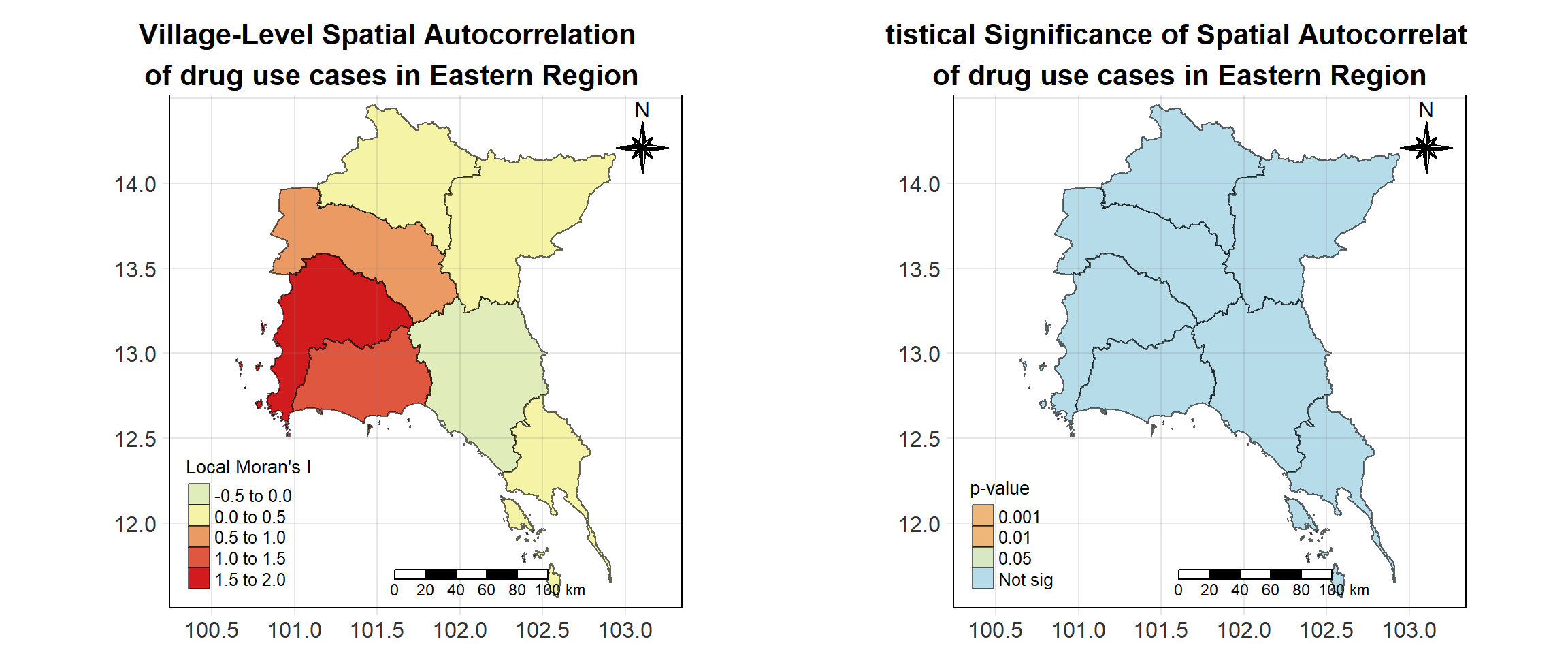

Southern Region

southern_local <- tm_shape(southern_lisa_2017)+
  tm_fill("ii", 
          palette = c("#e1ecbb","#f5f3a6", "#ec9a64","#de573e","#d21b1c"),
          title = "Local Moran's I",
          midpoint = NA) +
  tm_borders(col = "black", alpha = 0.6)+
  tm_layout(main.title = "Village-Level Spatial Autocorrelation \nof drug use cases in Southern Region",
            main.title.position = "center",
            main.title.size = 1.3,
            main.title.fontface = "bold",
            legend.title.size = 1,
            legend.text.size = 0.8,
            frame = TRUE) +
  tm_borders(alpha = 0.5) +
  tm_compass(type="8star", text.size = 1, size = 2, position=c("RIGHT", "TOP")) +
  tm_scale_bar(position=c("LEFT", "BOTTOM"), text.size=1) +
  tm_grid(labels.size = 1,alpha =0.2)

southern_sig <- tm_shape(southern_lisa_2017)+
  tm_fill("p_ii_sim", 
          palette = c("#d21b1c","#ec9a64","#f5f3a6","#c9e3d2","#b7dce9"),
          breaks = c(0, 0.001, 0.01, 0.05, 1),
          labels = c("0.001", "0.01", "0.05", "Not sig"), 
          title = "p-value",
          midpoint = NA) +
  tm_borders(col = "black", alpha = 0.6)+
  tm_layout(main.title = "Statistical Significance of Spatial Autocorrelation\n of drug use cases in Southern Region",
            main.title.position = "center",
            main.title.size = 1.3,
            main.title.fontface = "bold",
            legend.title.size = 1,
            legend.text.size = 0.8,
            frame = TRUE) +
  tm_borders(alpha = 0.5) +
  tm_compass(type="8star", text.size = 1, size = 2, position=c("RIGHT", "TOP")) +
  tm_scale_bar(position=c("LEFT", "BOTTOM"), text.size=1) +
  tm_grid(labels.size = 1,alpha =0.2)

tmap_arrange(southern_local,southern_sig, asp=1, ncol=2)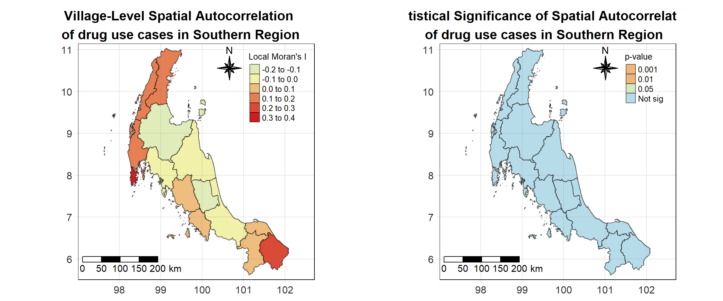

Analysis & Discussion

# Create the second map for northeastern_lisa_2017
northeastern_map <- tm_shape(northeastern_lisa_2017) +
  tm_polygons(id="label") +
  tm_borders(col = "black", alpha = 0.6) +
  tm_shape(northeastern_lisa_2017_sig) +
  tm_fill("mean", 
          palette = c("#b7dce9","#ec9a64","#e1ecbb", "#d21b1c"),
          title = "LISA class",
          midpoint = NA,
          legend.hist = TRUE, 
          legend.is.portrait = TRUE,
          legend.hist.z = 0.5) +
  tm_borders(col = "black", alpha = 0.6) +
  tm_layout(main.title = "2017 LISA plot of northeastern region",
            main.title.size = 0.8,
            legend.outside = TRUE)

# Create the first map for central_lisa_2017
central_map <- tm_shape(central_lisa_2017) +
  tm_polygons(id="label") +
  tm_borders(col = "black", alpha = 0.6) +
  tm_shape(central_lisa_2017_sig) +
  tm_fill("mean", 
          palette = c("#b7dce9","#ec9a64","#e1ecbb", "#d21b1c"),
          title = "LISA class",
          midpoint = NA,
          legend.hist = TRUE, 
          legend.is.portrait = TRUE,
          legend.hist.z = 0.5) +
  tm_borders(col = "black", alpha = 0.6) +
  tm_layout(main.title = "2017 LISA plot of central region",
            main.title.size = 0.8,
            legend.outside = TRUE)

# Arrange the two maps side by side
tmap_arrange(northeastern_map, central_map, asp=1, ncol=2)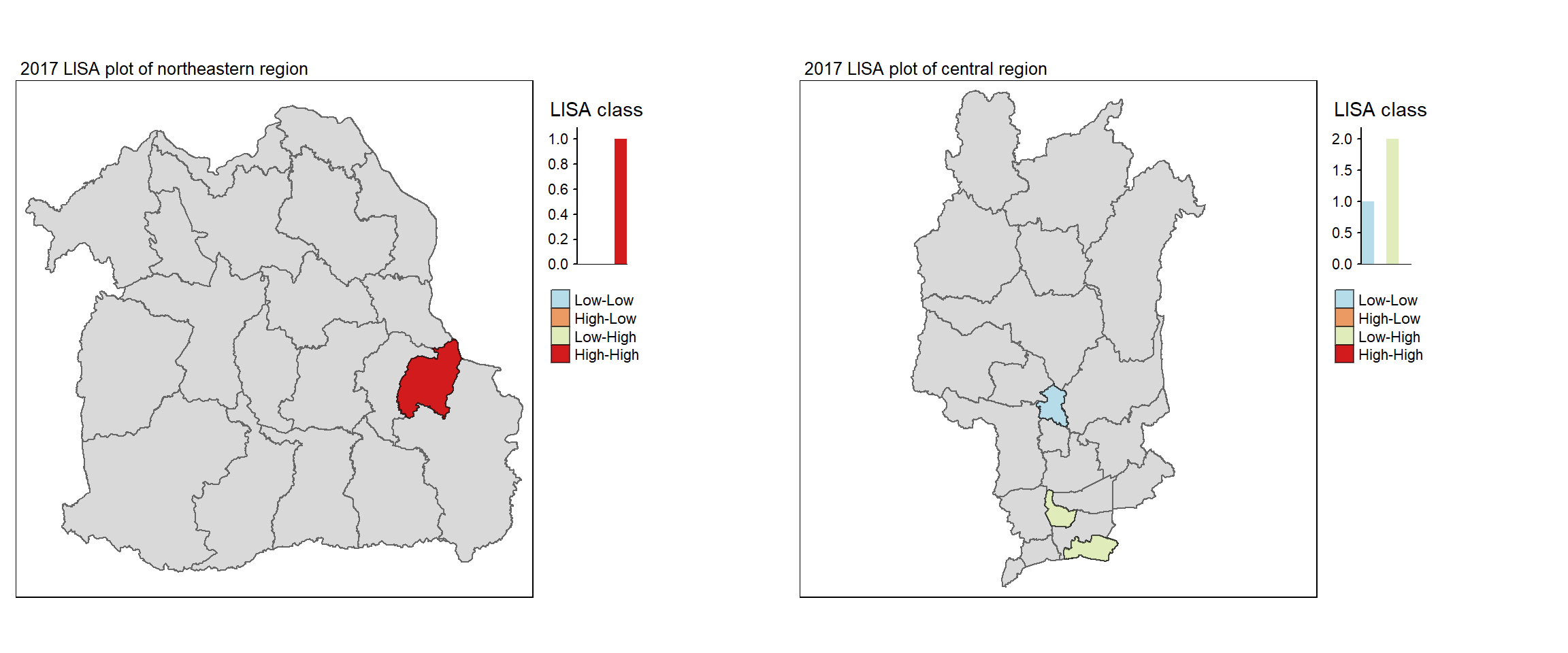

Within the year 2017, the northeastern and central regions of Thailand present an intriguing spatial autocorrelation pattern characterized by the co-existence of Low-Low and Low-High clusters in the central region, and High-High clusters in the northeastern region.

In contrast, the Northeastern region (left plot) shows a pronounced High-High cluster in the eastern border provinces, where both the province and its neighbors experience high rates of drug use. This significant clustering highlights a potential hotspot in the northeastern part of Thailand, indicating areas that may require targeted interventions for drug-related issues.

In the Central region (right plot), we observe a combination of Low-Low clusters in the province of Singburi, where areas with low drug use rates are surrounded by similarly low-use neighbors, and Low-High clusters in the south, where provinces with higher drug use rates are adjacent to those with lower rates. This pattern suggests a transitional area where drug use may be increasing, potentially influenced by neighboring provinces that are experiencing higher levels of drug-related incidents. The close proximity could indicate a spillover effect, notably into the provinces of Nonthaburi and Samut Prakan, highlighting the importance of monitoring and addressing drug use in these interconnected areas to prevent further escalation. Overall, the central region’s mixed clustering patterns reveal a complex landscape of drug use, necessitating tailored strategies for intervention and prevention.

Year 2018

northeastern_lisa_2018 <- lisa_2018 %>% filter(province_en %in% northeastern)
northern_lisa_2018 <- lisa_2018 %>% filter(province_en %in% northern)
western_lisa_2018 <- lisa_2018 %>% filter(province_en %in% western)
central_lisa_2018 <- lisa_2018 %>% filter(province_en %in% central)
eastern_lisa_2018 <- lisa_2018 %>% filter(province_en %in% eastern)
southern_lisa_2018 <- lisa_2018 %>% filter(province_en %in% southern)

northeastern_lisa_2018_sig <- lisa_2018_sig %>% filter(province_en %in% northeastern)
northern_lisa_2018_sig <- lisa_2018_sig %>% filter(province_en %in% northern)
western_lisa_2018_sig <- lisa_2018_sig %>% filter(province_en %in% western)
central_lisa_2018_sig <- lisa_2018_sig %>% filter(province_en %in% central)
eastern_lisa_2018_sig <- lisa_2018_sig %>% filter(province_en %in% eastern)
southern_lisa_2018_sig <- lisa_2018_sig %>% filter(province_en %in% southern)

Northeastern Region

northeastern_local <- tm_shape(northeastern_lisa_2018)+
  tm_fill("ii", 
          palette = c("#e1ecbb","#f5f3a6", "#ec9a64","#de573e","#d21b1c"),
          title = "Local Moran's I",
          midpoint = NA) +
  tm_borders(col = "black", alpha = 0.6)+
  tm_layout(main.title = "Village-Level Spatial Autocorrelation \nof drug use cases in Northeastern Region",
            main.title.position = "center",
            main.title.size = 1.3,
            main.title.fontface = "bold",
            legend.title.size = 1,
            legend.text.size = 0.8,
            frame = TRUE) +
  tm_borders(alpha = 0.5) +
  tm_compass(type="8star", text.size = 1, size = 2, position=c("RIGHT", "TOP")) +
  tm_scale_bar(position=c("LEFT", "BOTTOM"), text.size=1) +
  tm_grid(labels.size = 1,alpha =0.2)

northeastern_sig <- tm_shape(northeastern_lisa_2018)+
  tm_fill("p_ii_sim", 
          palette = c("#d21b1c","#ec9a64","#f5f3a6","#c9e3d2","#b7dce9"),
          breaks = c(0, 0.001, 0.01, 0.05, 1),
          labels = c("0.001", "0.01", "0.05", "Not sig"), 
          title = "p-value",
          midpoint = NA) +
  tm_borders(col = "black", alpha = 0.6)+
  tm_layout(main.title = "Statistical Significance of Spatial Autocorrelation\n of drug use cases in Northeastern Region",
            main.title.position = "center",
            main.title.size = 1.3,
            main.title.fontface = "bold",
            legend.title.size = 1,
            legend.text.size = 0.8,
            frame = TRUE) +
  tm_borders(alpha = 0.5) +
  tm_compass(type="8star", text.size = 1, size = 2, position=c("RIGHT", "TOP")) +
  tm_scale_bar(position=c("LEFT", "BOTTOM"), text.size=1) +
  tm_grid(labels.size = 1,alpha =0.2)

tmap_arrange(northeastern_local,northeastern_sig, asp=1, ncol=2)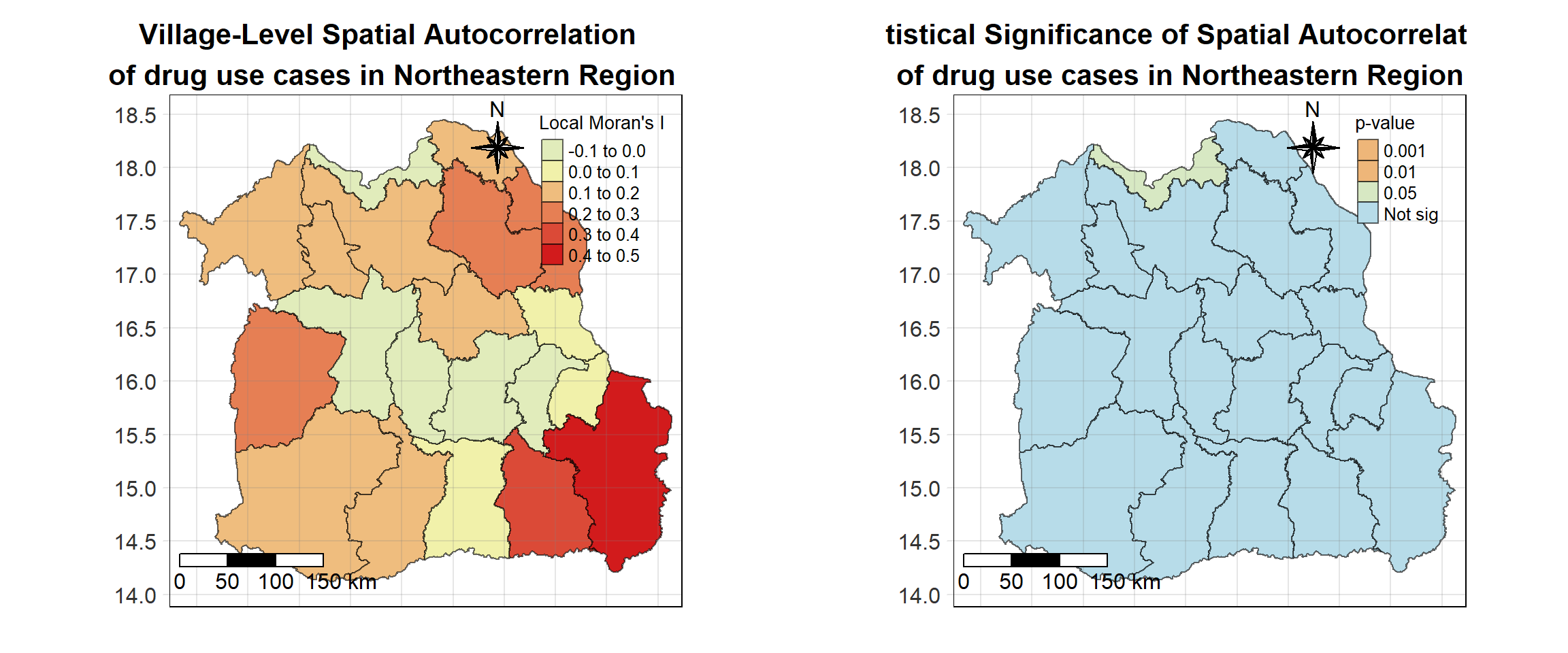

Northern Region

northern_local <- tm_shape(northern_lisa_2018)+
  tm_fill("ii", 
          palette = c("#e1ecbb","#f5f3a6", "#ec9a64","#de573e","#d21b1c"),
          title = "Local Moran's I",
          midpoint = NA) +
  tm_borders(col = "black", alpha = 0.6)+
  tm_layout(main.title = "Village-Level Spatial Autocorrelation \nof drug use cases in Northern Region",
            main.title.position = "center",
            main.title.size = 1.3,
            main.title.fontface = "bold",
            legend.title.size = 1,
            legend.text.size = 0.8,
            frame = TRUE) +
  tm_borders(alpha = 0.5) +
  tm_compass(type="8star", text.size = 1, size = 2, position=c("RIGHT", "TOP")) +
  tm_scale_bar(position=c("LEFT", "BOTTOM"), text.size=1) +
  tm_grid(labels.size = 1,alpha =0.2)

northern_sig <- tm_shape(northern_lisa_2018)+
  tm_fill("p_ii_sim", 
          palette = c("#d21b1c","#ec9a64","#f5f3a6","#c9e3d2","#b7dce9"),
          breaks = c(0, 0.001, 0.01, 0.05, 1),
          labels = c("0.001", "0.01", "0.05", "Not sig"), 
          title = "p-value",
          midpoint = NA) +
  tm_borders(col = "black", alpha = 0.6)+
  tm_layout(main.title = "Statistical Significance of Spatial Autocorrelation\n of drug use cases in Northern Region",
            main.title.position = "center",
            main.title.size = 1.3,
            main.title.fontface = "bold",
            legend.title.size = 1,
            legend.text.size = 0.8,
            frame = TRUE) +
  tm_borders(alpha = 0.5) +
  tm_compass(type="8star", text.size = 1, size = 2, position=c("RIGHT", "TOP")) +
  tm_scale_bar(position=c("LEFT", "BOTTOM"), text.size=1) +
  tm_grid(labels.size = 1,alpha =0.2)

tmap_arrange(northern_local,northern_sig, asp=1, ncol=2)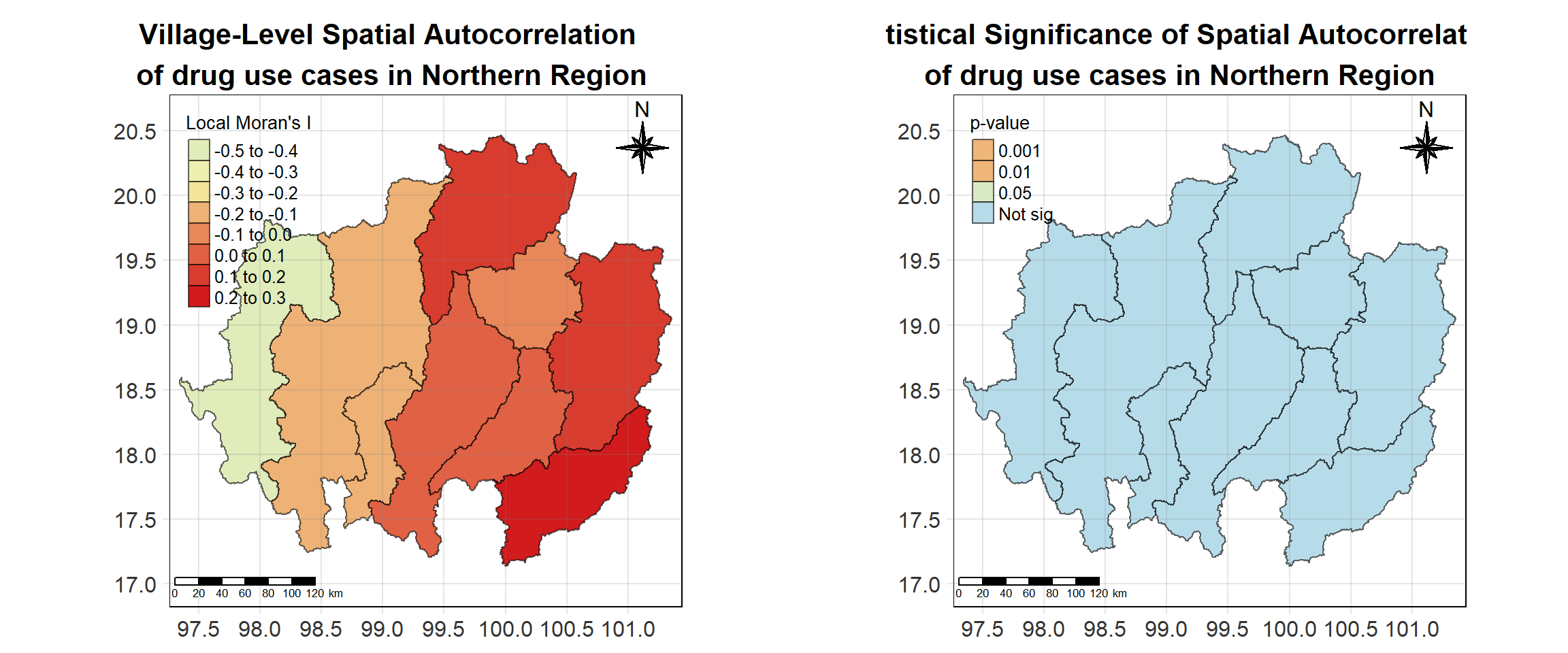

Western Region

western_local <- tm_shape(western_lisa_2018)+
  tm_fill("ii", 
          palette = c("#e1ecbb","#f5f3a6", "#ec9a64","#de573e","#d21b1c"),
          title = "Local Moran's I",
          midpoint = NA) +
  tm_borders(col = "black", alpha = 0.6)+
  tm_layout(main.title = "Village-Level Spatial Autocorrelation \nof drug use cases in Western Region",
            main.title.position = "center",
            main.title.size = 1.3,
            main.title.fontface = "bold",
            legend.title.size = 1,
            legend.text.size = 0.8,
            frame = TRUE) +
  tm_borders(alpha = 0.5) +
  tm_compass(type="8star", text.size = 1, size = 2, position=c("RIGHT", "TOP")) +
  tm_scale_bar(position=c("LEFT", "BOTTOM"), text.size=1) +
  tm_grid(labels.size = 1,alpha =0.2)

western_sig <- tm_shape(western_lisa_2018)+
  tm_fill("p_ii_sim", 
          palette = c("#d21b1c","#ec9a64","#f5f3a6","#c9e3d2","#b7dce9"),
          breaks = c(0, 0.001, 0.01, 0.05, 1),
          labels = c("0.001", "0.01", "0.05", "Not sig"), 
          title = "p-value",
          midpoint = NA) +
  tm_borders(col = "black", alpha = 0.6)+
  tm_layout(main.title = "Statistical Significance of Spatial Autocorrelation\n of drug use cases in Western Region",
            main.title.position = "center",
            main.title.size = 1.3,
            main.title.fontface = "bold",
            legend.title.size = 1,
            legend.text.size = 0.8,
            frame = TRUE) +
  tm_borders(alpha = 0.5) +
  tm_compass(type="8star", text.size = 1, size = 2, position=c("RIGHT", "TOP")) +
  tm_scale_bar(position=c("LEFT", "BOTTOM"), text.size=1) +
  tm_grid(labels.size = 1,alpha =0.2)

tmap_arrange(western_local,western_sig, asp=1, ncol=2)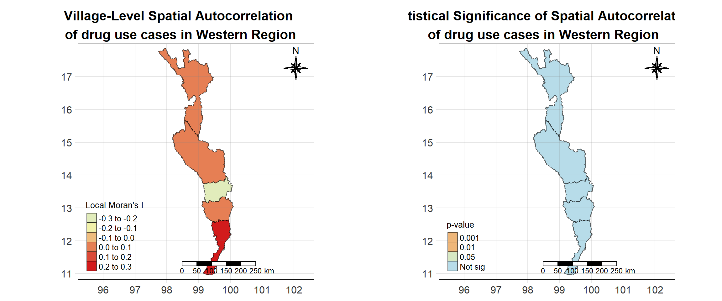

Central Region

central_local <- tm_shape(central_lisa_2018)+
  tm_fill("ii", 
          palette = c("#e1ecbb","#f5f3a6", "#ec9a64","#de573e","#d21b1c"),
          title = "Local Moran's I",
          midpoint = NA) +
  tm_borders(col = "black", alpha = 0.6)+
  tm_layout(main.title = "Village-Level Spatial Autocorrelation \nof drug use cases in Central Region",
            main.title.position = "center",
            main.title.size = 1.3,
            main.title.fontface = "bold",
            legend.title.size = 1,
            legend.text.size = 0.8,
            frame = TRUE) +
  tm_borders(alpha = 0.5) +
  tm_compass(type="8star", text.size = 1, size = 2, position=c("RIGHT", "TOP")) +
  tm_scale_bar(position=c("LEFT", "BOTTOM"), text.size=1) +
  tm_grid(labels.size = 1,alpha =0.2)

central_sig <- tm_shape(central_lisa_2018)+
  tm_fill("p_ii_sim", 
          palette = c("#d21b1c","#ec9a64","#f5f3a6","#c9e3d2","#b7dce9"),
          breaks = c(0, 0.001, 0.01, 0.05, 1),
          labels = c("0.001", "0.01", "0.05", "Not sig"), 
          title = "p-value",
          midpoint = NA) +
  tm_borders(col = "black", alpha = 0.6)+
  tm_layout(main.title = "Statistical Significance of Spatial Autocorrelation\n of drug use cases in Central Region",
            main.title.position = "center",
            main.title.size = 1.3,
            main.title.fontface = "bold",
            legend.title.size = 1,
            legend.text.size = 0.8,
            frame = TRUE) +
  tm_borders(alpha = 0.5) +
  tm_compass(type="8star", text.size = 1, size = 2, position=c("RIGHT", "TOP")) +
  tm_scale_bar(position=c("LEFT", "BOTTOM"), text.size=1) +
  tm_grid(labels.size = 1,alpha =0.2)

tmap_arrange(central_local,central_sig, asp=1, ncol=2)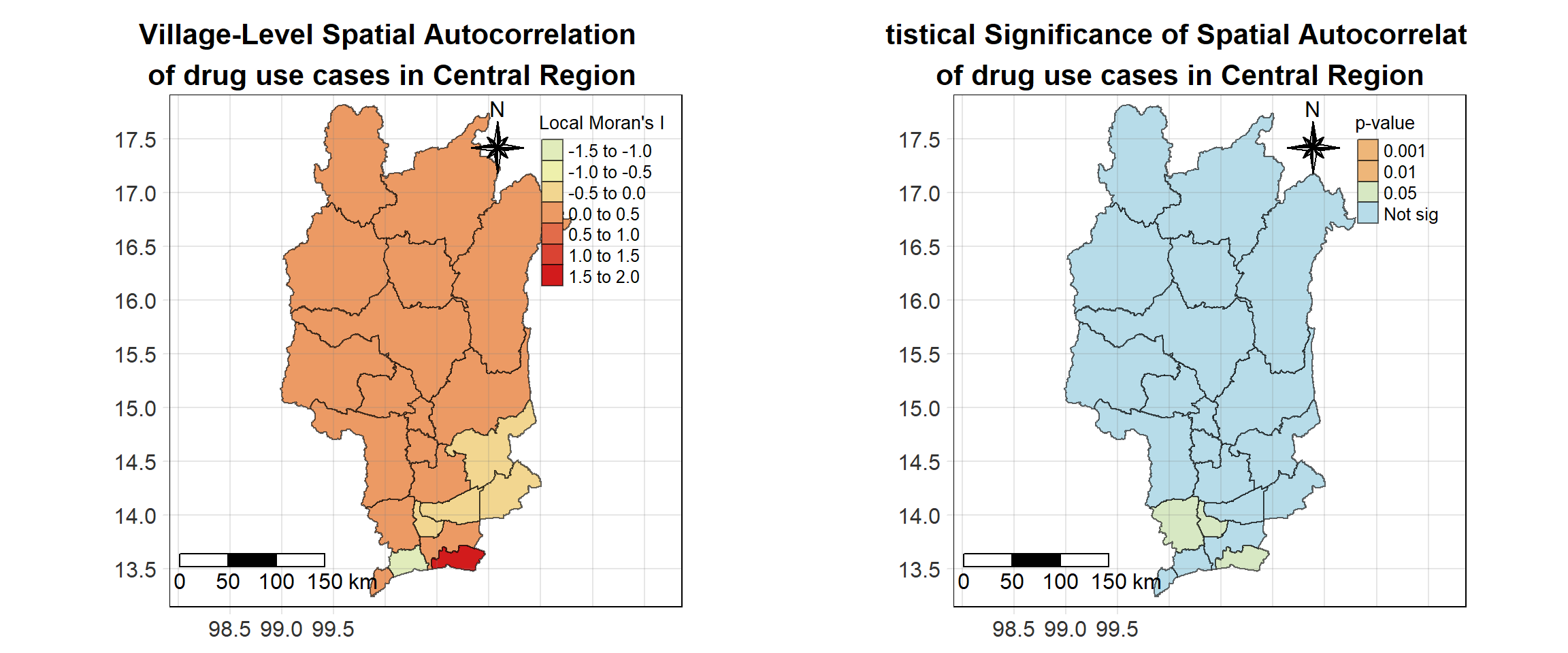

Eastern Region

eastern_local <- tm_shape(eastern_lisa_2018)+
  tm_fill("ii", 
          palette = c("#e1ecbb","#f5f3a6", "#ec9a64","#de573e","#d21b1c"),
          title = "Local Moran's I",
          midpoint = NA) +
  tm_borders(col = "black", alpha = 0.6)+
  tm_layout(main.title = "Village-Level Spatial Autocorrelation \nof drug use cases in Eastern Region",
            main.title.position = "center",
            main.title.size = 1.3,
            main.title.fontface = "bold",
            legend.title.size = 1,
            legend.text.size = 0.8,
            frame = TRUE) +
  tm_borders(alpha = 0.5) +
  tm_compass(type="8star", text.size = 1, size = 2, position=c("RIGHT", "TOP")) +
  tm_scale_bar(position=c("LEFT", "BOTTOM"), text.size=1) +
  tm_grid(labels.size = 1,alpha =0.2)

eastern_sig <- tm_shape(eastern_lisa_2018)+
  tm_fill("p_ii_sim", 
          palette = c("#d21b1c","#ec9a64","#f5f3a6","#c9e3d2","#b7dce9"),
          breaks = c(0, 0.001, 0.01, 0.05, 1),
          labels = c("0.001", "0.01", "0.05", "Not sig"), 
          title = "p-value",
          midpoint = NA) +
  tm_borders(col = "black", alpha = 0.6)+
  tm_layout(main.title = "Statistical Significance of Spatial Autocorrelation\n of drug use cases in Eastern Region",
            main.title.position = "center",
            main.title.size = 1.3,
            main.title.fontface = "bold",
            legend.title.size = 1,
            legend.text.size = 0.8,
            frame = TRUE) +
  tm_borders(alpha = 0.5) +
  tm_compass(type="8star", text.size = 1, size = 2, position=c("RIGHT", "TOP")) +
  tm_scale_bar(position=c("LEFT", "BOTTOM"), text.size=1) +
  tm_grid(labels.size = 1,alpha =0.2)

tmap_arrange(eastern_local,eastern_sig, asp=1, ncol=2)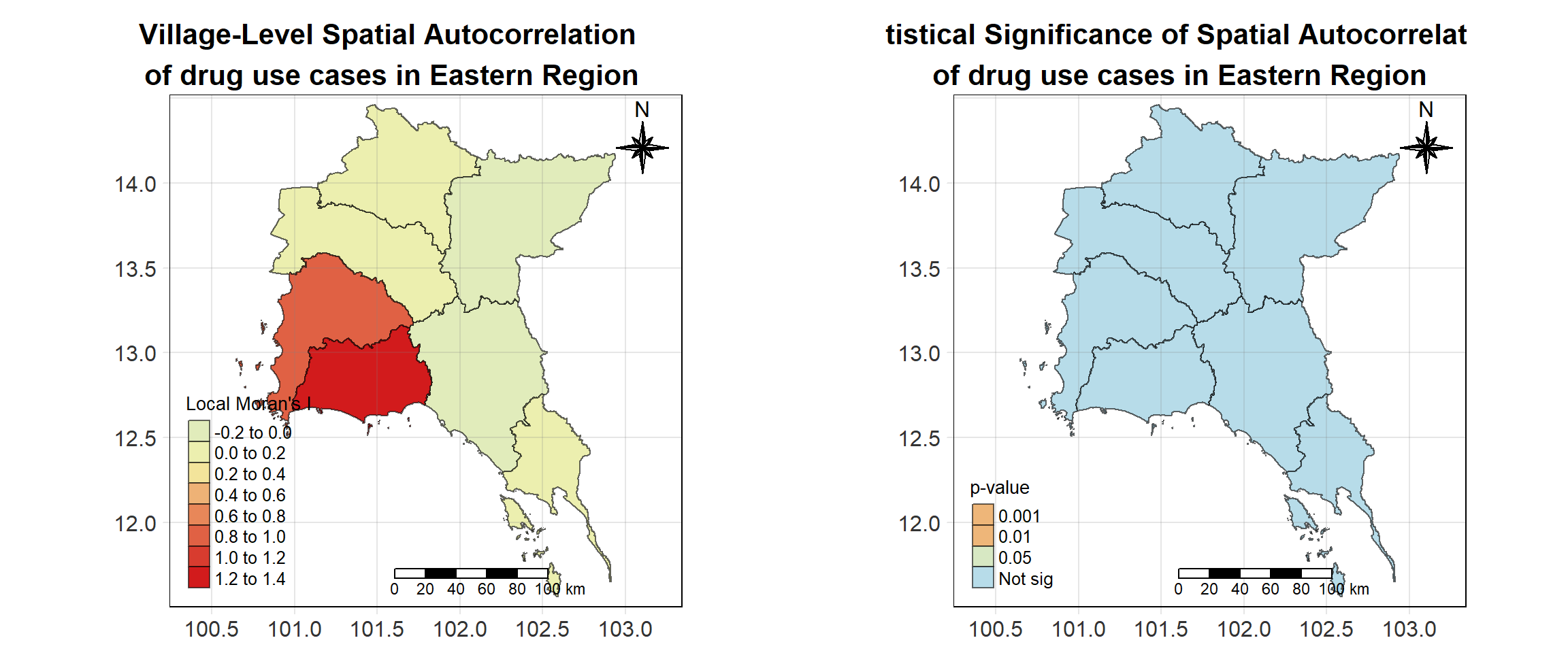

Southern Region

southern_local <- tm_shape(southern_lisa_2018)+
  tm_fill("ii", 
          palette = c("#e1ecbb","#f5f3a6", "#ec9a64","#de573e","#d21b1c"),
          title = "Local Moran's I",
          midpoint = NA) +
  tm_borders(col = "black", alpha = 0.6)+
  tm_layout(main.title = "Village-Level Spatial Autocorrelation \nof drug use cases in Southern Region",
            main.title.position = "center",
            main.title.size = 1.3,
            main.title.fontface = "bold",
            legend.title.size = 1,
            legend.text.size = 0.8,
            frame = TRUE) +
  tm_borders(alpha = 0.5) +
  tm_compass(type="8star", text.size = 1, size = 2, position=c("RIGHT", "TOP")) +
  tm_scale_bar(position=c("LEFT", "BOTTOM"), text.size=1) +
  tm_grid(labels.size = 1,alpha =0.2)

southern_sig <- tm_shape(southern_lisa_2018)+
  tm_fill("p_ii_sim", 
          palette = c("#d21b1c","#ec9a64","#f5f3a6","#c9e3d2","#b7dce9"),
          breaks = c(0, 0.001, 0.01, 0.05, 1),
          labels = c("0.001", "0.01", "0.05", "Not sig"), ,
          title = "p-value",
          midpoint = NA) +
  tm_borders(col = "black", alpha = 0.6)+
  tm_layout(main.title = "Statistical Significance of Spatial Autocorrelation\n of drug use cases in Southern Region",
            main.title.position = "center",
            main.title.size = 1.3,
            main.title.fontface = "bold",
            legend.title.size = 1,
            legend.text.size = 0.8,
            frame = TRUE) +
  tm_borders(alpha = 0.5) +
  tm_compass(type="8star", text.size = 1, size = 2, position=c("RIGHT", "TOP")) +
  tm_scale_bar(position=c("LEFT", "BOTTOM"), text.size=1) +
  tm_grid(labels.size = 1,alpha =0.2)

tmap_arrange(southern_local,southern_sig, asp=1, ncol=2)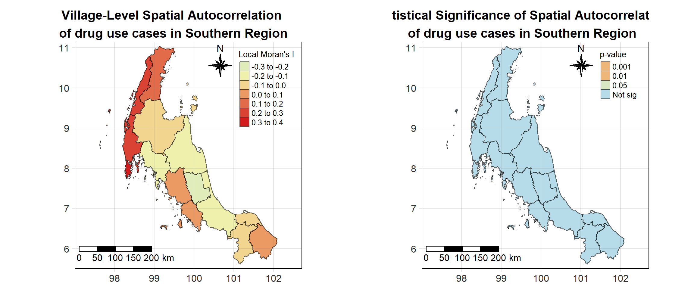

Analysis & Discussion

# Create the second map for northeastern_lisa_2018
northeastern_map <- tm_shape(northeastern_lisa_2018) +
  tm_polygons(id="label") +
  tm_borders(col = "black", alpha = 0.6) +
  tm_shape(northeastern_lisa_2018_sig) +
  tm_fill("mean", 
          palette = c("#b7dce9","#ec9a64","#e1ecbb", "#d21b1c"),
          title = "LISA class",
          midpoint = NA,
          legend.hist = TRUE, 
          legend.is.portrait = TRUE,
          legend.hist.z = 0.5) +
  tm_borders(col = "black", alpha = 0.6) +
  tm_layout(main.title = "2018 LISA plot of northeastern region",
            main.title.size = 0.8,
            legend.outside = TRUE)

# Create the first map for central_lisa_2018
central_map <- tm_shape(central_lisa_2018) +
  tm_polygons(id="label") +
  tm_borders(col = "black", alpha = 0.6) +
  tm_shape(central_lisa_2018_sig) +
  tm_fill("mean", 
          palette = c("#b7dce9","#ec9a64","#e1ecbb", "#d21b1c"),
          title = "LISA class",
          midpoint = NA,
          legend.hist = TRUE, 
          legend.is.portrait = TRUE,
          legend.hist.z = 0.5) +
  tm_borders(col = "black", alpha = 0.6) +
  tm_layout(main.title = "2018 LISA plot of central region",
            main.title.size = 0.8,
            legend.outside = TRUE)

# Arrange the two maps side by side
tmap_arrange(northeastern_map, central_map, asp=1, ncol=2)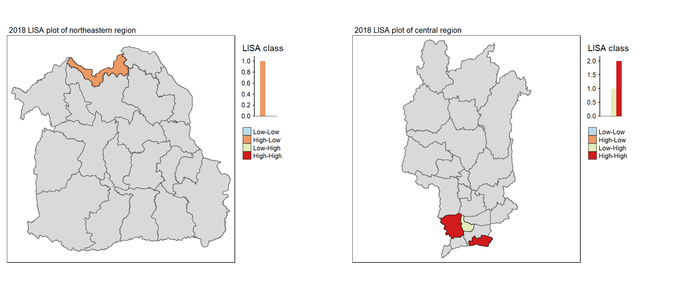

In 2018, the spatial autocorrelation patterns in the northeastern and central regions of Thailand reveal notable shifts in the classification of drug use incidents compared to the previous year.

In the Northeastern region (left plot), we observe a significant presence of High-Low clusters, particularly in the northern provinces. This indicates that areas with high drug use rates are bordered by regions with lower rates, suggesting a potential influence or spillover effect where increased drug activity in some areas may affect their neighbors. The rest of the region largely remains unclassified, highlighting a shift in the drug use dynamics in this area.

Conversely, in the Central region (right plot), there is a noticeable increase in High-High clusters, especially in the southern provinces, where areas with high drug use rates are surrounded by similarly high-use neighbors. This indicates that drug-related issues may be more concentrated in these provinces, necessitating targeted interventions to address the growing problem. Additionally, Low-Low clusters can be seen in some provinces, where low drug use rates are observed alongside similarly low-use areas, signifying pockets of stability amidst rising drug use in surrounding regions.

Overall, both regions illustrate the evolving landscape of drug use in Thailand in 2018, emphasizing the importance of spatial analysis in understanding and responding to changing patterns in drug-related incidents. The identification of clusters can inform policy decisions and resource allocation for effective intervention strategies.

Year 2019

northeastern_lisa_2019 <- lisa_2019 %>% filter(province_en %in% northeastern)
northern_lisa_2019 <- lisa_2019 %>% filter(province_en %in% northern)
western_lisa_2019 <- lisa_2019 %>% filter(province_en %in% western)
central_lisa_2019 <- lisa_2019 %>% filter(province_en %in% central)
eastern_lisa_2019 <- lisa_2019 %>% filter(province_en %in% eastern)
southern_lisa_2019 <- lisa_2019 %>% filter(province_en %in% southern)

northeastern_lisa_2019_sig <- lisa_2019_sig %>% filter(province_en %in% northeastern)
northern_lisa_2019_sig <- lisa_2019_sig %>% filter(province_en %in% northern)
western_lisa_2019_sig <- lisa_2019_sig %>% filter(province_en %in% western)
central_lisa_2019_sig <- lisa_2019_sig %>% filter(province_en %in% central)
eastern_lisa_2019_sig <- lisa_2019_sig %>% filter(province_en %in% eastern)
southern_lisa_2019_sig <- lisa_2019_sig %>% filter(province_en %in% southern)

Northeastern Region

northeastern_local <- tm_shape(northeastern_lisa_2019)+
  tm_fill("ii", 
          palette = c("#e1ecbb","#f5f3a6", "#ec9a64","#de573e","#d21b1c"),
          title = "Local Moran's I",
          midpoint = NA) +
  tm_borders(col = "black", alpha = 0.6)+
  tm_layout(main.title = "Village-Level Spatial Autocorrelation \nof drug use cases in Northeastern Region",
            main.title.position = "center",
            main.title.size = 1.3,
            main.title.fontface = "bold",
            legend.title.size = 1,
            legend.text.size = 0.8,
            frame = TRUE) +
  tm_borders(alpha = 0.5) +
  tm_compass(type="8star", text.size = 1, size = 2, position=c("RIGHT", "TOP")) +
  tm_scale_bar(position=c("LEFT", "BOTTOM"), text.size=1) +
  tm_grid(labels.size = 1,alpha =0.2)

northeastern_sig <- tm_shape(northeastern_lisa_2019)+
  tm_fill("p_ii_sim", 
          palette = c("#d21b1c","#ec9a64","#f5f3a6","#c9e3d2","#b7dce9"),
          breaks = c(0, 0.001, 0.01, 0.05, 1),
          labels = c("0.001", "0.01", "0.05", "Not sig"), 
          title = "p-value",
          midpoint = NA) +
  tm_borders(col = "black", alpha = 0.6)+
  tm_layout(main.title = "Statistical Significance of Spatial Autocorrelation\n of drug use cases in Northeastern Region",
            main.title.position = "center",
            main.title.size = 1.3,
            main.title.fontface = "bold",
            legend.title.size = 1,
            legend.text.size = 0.8,
            frame = TRUE) +
  tm_borders(alpha = 0.5) +
  tm_compass(type="8star", text.size = 1, size = 2, position=c("RIGHT", "TOP")) +
  tm_scale_bar(position=c("LEFT", "BOTTOM"), text.size=1) +
  tm_grid(labels.size = 1,alpha =0.2)

tmap_arrange(northeastern_local,northeastern_sig, asp=1, ncol=2)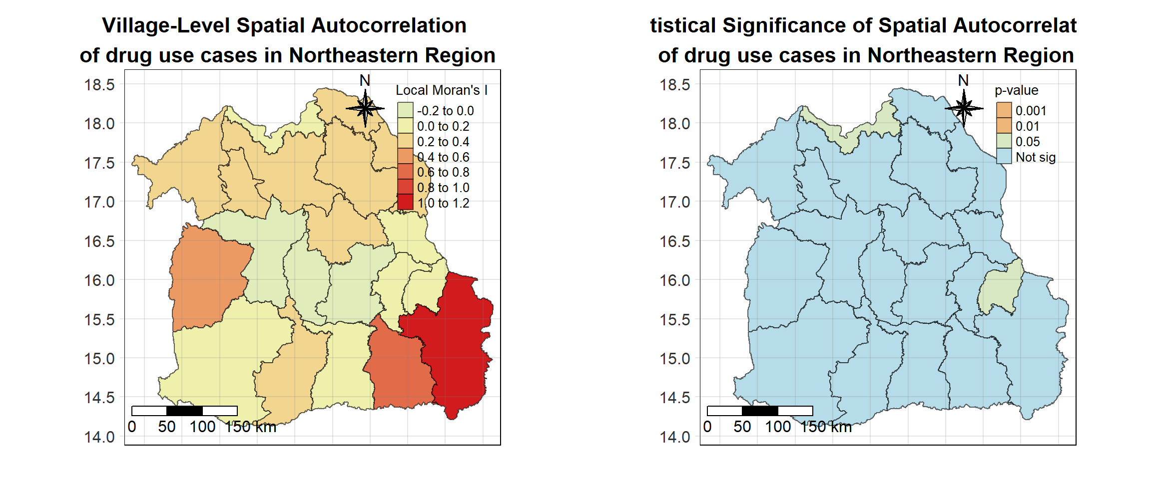

Northern Region

northern_local <- tm_shape(northern_lisa_2019)+
  tm_fill("ii", 
          palette = c("#e1ecbb","#f5f3a6", "#ec9a64","#de573e","#d21b1c"),
          title = "Local Moran's I",
          midpoint = NA) +
  tm_borders(col = "black", alpha = 0.6)+
  tm_layout(main.title = "Village-Level Spatial Autocorrelation \nof drug use cases in Northern Region",
            main.title.position = "center",
            main.title.size = 1.3,
            main.title.fontface = "bold",
            legend.title.size = 1,
            legend.text.size = 0.8,
            frame = TRUE) +
  tm_borders(alpha = 0.5) +
  tm_compass(type="8star", text.size = 1, size = 2, position=c("RIGHT", "TOP")) +
  tm_scale_bar(position=c("LEFT", "BOTTOM"), text.size=1) +
  tm_grid(labels.size = 1,alpha =0.2)

northern_sig <- tm_shape(northern_lisa_2019)+
  tm_fill("p_ii_sim", 
          palette = c("#d21b1c","#ec9a64","#f5f3a6","#c9e3d2","#b7dce9"),
          breaks = c(0, 0.001, 0.01, 0.05, 1),
          labels = c("0.001", "0.01", "0.05", "Not sig"), 
          title = "p-value",
          midpoint = NA) +
  tm_borders(col = "black", alpha = 0.6)+
  tm_layout(main.title = "Statistical Significance of Spatial Autocorrelation\n of drug use cases in Northern Region",
            main.title.position = "center",
            main.title.size = 1.3,
            main.title.fontface = "bold",
            legend.title.size = 1,
            legend.text.size = 0.8,
            frame = TRUE) +
  tm_borders(alpha = 0.5) +
  tm_compass(type="8star", text.size = 1, size = 2, position=c("RIGHT", "TOP")) +
  tm_scale_bar(position=c("LEFT", "BOTTOM"), text.size=1) +
  tm_grid(labels.size = 1,alpha =0.2)

tmap_arrange(northern_local,northern_sig, asp=1, ncol=2)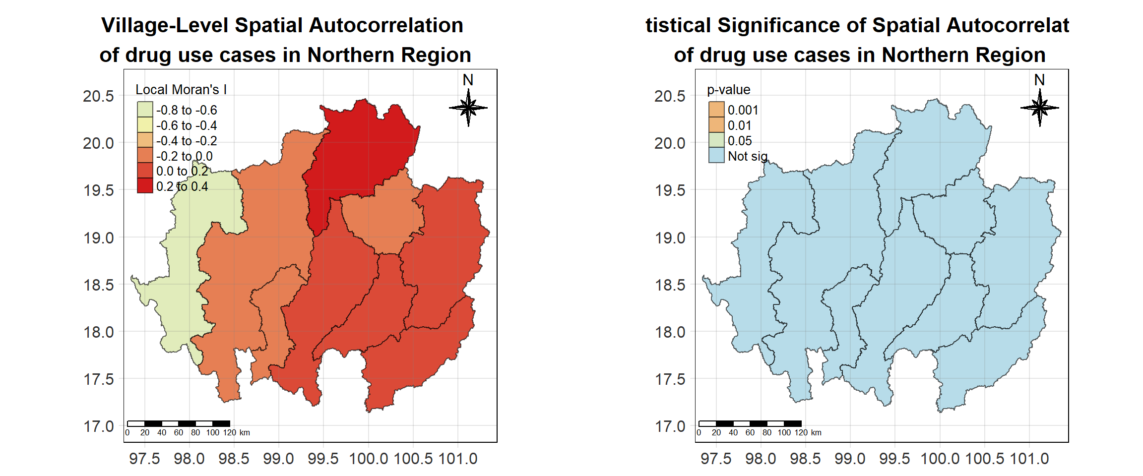

Western Region

western_local <- tm_shape(western_lisa_2019)+
  tm_fill("ii", 
          palette = c("#e1ecbb","#f5f3a6", "#ec9a64","#de573e","#d21b1c"),
          title = "Local Moran's I",
          midpoint = NA) +
  tm_borders(col = "black", alpha = 0.6)+
  tm_layout(main.title = "Village-Level Spatial Autocorrelation \nof drug use cases in Western Region",
            main.title.position = "center",
            main.title.size = 1.3,
            main.title.fontface = "bold",
            legend.title.size = 1,
            legend.text.size = 0.8,
            frame = TRUE) +
  tm_borders(alpha = 0.5) +
  tm_compass(type="8star", text.size = 1, size = 2, position=c("RIGHT", "TOP")) +
  tm_scale_bar(position=c("LEFT", "BOTTOM"), text.size=1) +
  tm_grid(labels.size = 1,alpha =0.2)

western_sig <- tm_shape(western_lisa_2019)+
  tm_fill("p_ii_sim", 
          palette = c("#d21b1c","#ec9a64","#f5f3a6","#c9e3d2","#b7dce9"),
          breaks = c(0, 0.001, 0.01, 0.05, 1),
          labels = c("0.001", "0.01", "0.05", "Not sig"), 
          title = "p-value",
          midpoint = NA) +
  tm_borders(col = "black", alpha = 0.6)+
  tm_layout(main.title = "Statistical Significance of Spatial Autocorrelation\n of drug use cases in Western Region",
            main.title.position = "center",
            main.title.size = 1.3,
            main.title.fontface = "bold",
            legend.title.size = 1,
            legend.text.size = 0.8,
            frame = TRUE) +
  tm_borders(alpha = 0.5) +
  tm_compass(type="8star", text.size = 1, size = 2, position=c("RIGHT", "TOP")) +
  tm_scale_bar(position=c("LEFT", "BOTTOM"), text.size=1) +
  tm_grid(labels.size = 1,alpha =0.2)

tmap_arrange(western_local,western_sig, asp=1, ncol=2)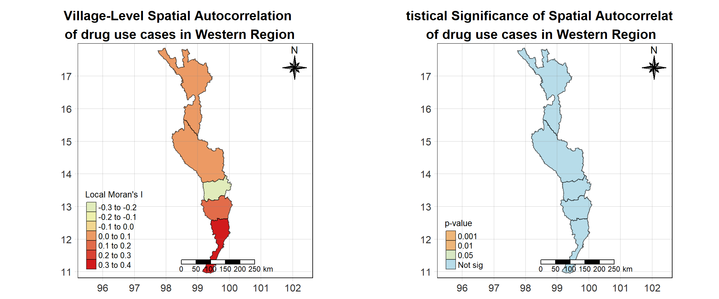

Central Region

central_local <- tm_shape(central_lisa_2019)+
  tm_fill("ii", 
          palette = c("#e1ecbb","#f5f3a6", "#ec9a64","#de573e","#d21b1c"),
          title = "Local Moran's I",
          midpoint = NA) +
  tm_borders(col = "black", alpha = 0.6)+
  tm_layout(main.title = "Village-Level Spatial Autocorrelation \nof drug use cases in North District",
            main.title.position = "center",
            main.title.size = 1.3,
            main.title.fontface = "bold",
            legend.title.size = 1,
            legend.text.size = 0.8,
            frame = TRUE) +
  tm_borders(alpha = 0.5) +
  tm_compass(type="8star", text.size = 1, size = 2, position=c("RIGHT", "TOP")) +
  tm_scale_bar(position=c("LEFT", "BOTTOM"), text.size=1) +
  tm_grid(labels.size = 1,alpha =0.2)

central_sig <- tm_shape(central_lisa_2019)+
  tm_fill("p_ii_sim", 
          palette = c("#d21b1c","#ec9a64","#f5f3a6","#c9e3d2","#b7dce9"),
          breaks = c(0, 0.001, 0.01, 0.05, 1),
          labels = c("0.001", "0.01", "0.05", "Not sig"), 
          title = "p-value",
          midpoint = NA) +
  tm_borders(col = "black", alpha = 0.6)+
  tm_layout(main.title = "Statistical Significance of Spatial Autocorrelation\n of drug use cases in North District",
            main.title.position = "center",
            main.title.size = 1.3,
            main.title.fontface = "bold",
            legend.title.size = 1,
            legend.text.size = 0.8,
            frame = TRUE) +
  tm_borders(alpha = 0.5) +
  tm_compass(type="8star", text.size = 1, size = 2, position=c("RIGHT", "TOP")) +
  tm_scale_bar(position=c("LEFT", "BOTTOM"), text.size=1) +
  tm_grid(labels.size = 1,alpha =0.2)

tmap_arrange(central_local,central_sig, asp=1, ncol=2)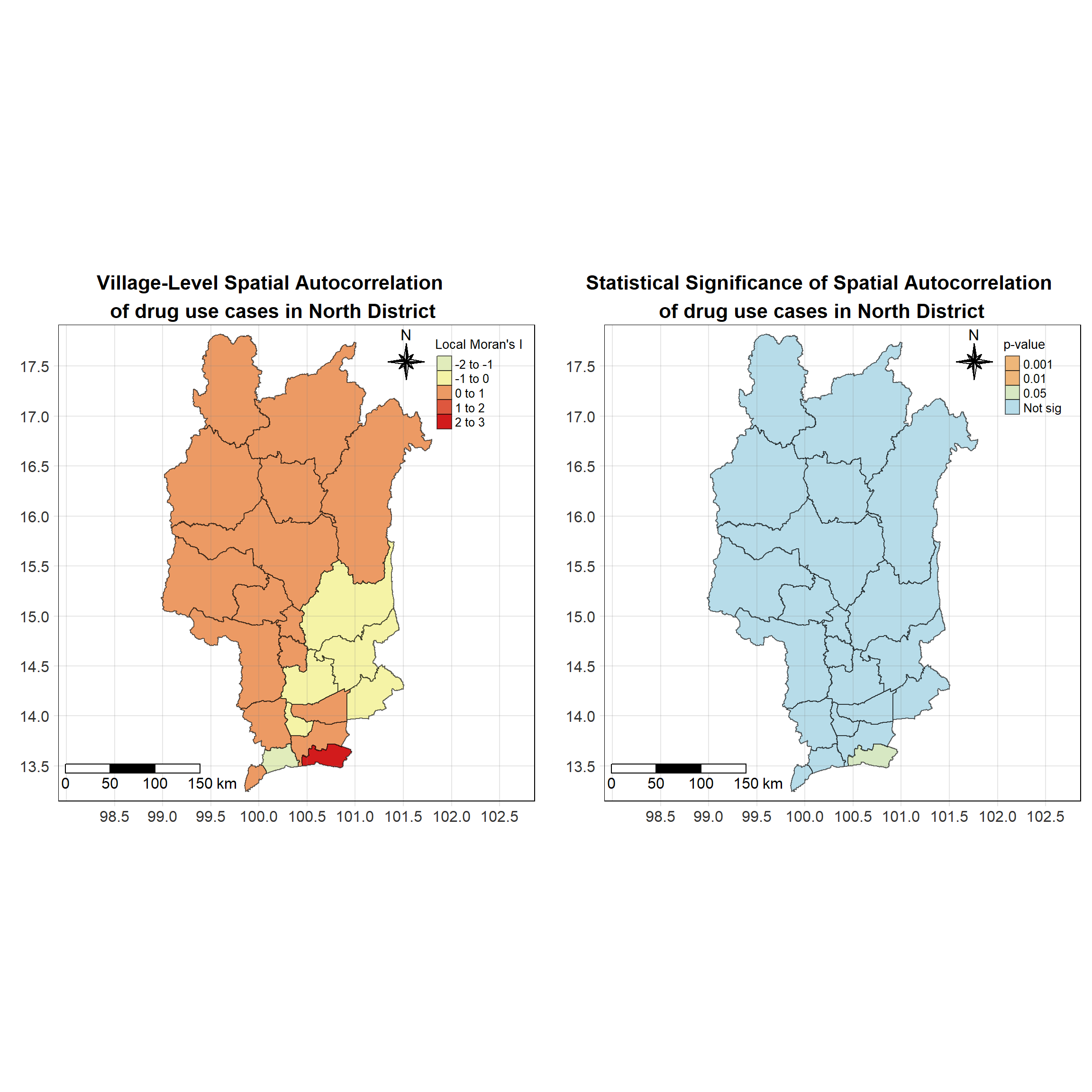

Eastern Region

eastern_local <- tm_shape(eastern_lisa_2019)+
  tm_fill("ii", 
          palette = c("#e1ecbb","#f5f3a6", "#ec9a64","#de573e","#d21b1c"),
          title = "Local Moran's I",
          midpoint = NA) +
  tm_borders(col = "black", alpha = 0.6)+
  tm_layout(main.title = "Village-Level Spatial Autocorrelation \nof drug use cases in Eastern Region",
            main.title.position = "center",
            main.title.size = 1.3,
            main.title.fontface = "bold",
            legend.title.size = 1,
            legend.text.size = 0.8,
            frame = TRUE) +
  tm_borders(alpha = 0.5) +
  tm_compass(type="8star", text.size = 1, size = 2, position=c("RIGHT", "TOP")) +
  tm_scale_bar(position=c("LEFT", "BOTTOM"), text.size=1) +
  tm_grid(labels.size = 1,alpha =0.2)

eastern_sig <- tm_shape(eastern_lisa_2019)+
  tm_fill("p_ii_sim", 
          palette = c("#d21b1c","#ec9a64","#f5f3a6","#c9e3d2","#b7dce9"),
          breaks = c(0, 0.001, 0.01, 0.05, 1),
          labels = c("0.001", "0.01", "0.05", "Not sig"), 
          title = "p-value",
          midpoint = NA) +
  tm_borders(col = "black", alpha = 0.6)+
  tm_layout(main.title = "Statistical Significance of Spatial Autocorrelation\n of drug use cases in Eastern Region",
            main.title.position = "center",
            main.title.size = 1.3,
            main.title.fontface = "bold",
            legend.title.size = 1,
            legend.text.size = 0.8,
            frame = TRUE) +
  tm_borders(alpha = 0.5) +
  tm_compass(type="8star", text.size = 1, size = 2, position=c("RIGHT", "TOP")) +
  tm_scale_bar(position=c("LEFT", "BOTTOM"), text.size=1) +
  tm_grid(labels.size = 1,alpha =0.2)

tmap_arrange(eastern_local,eastern_sig, asp=1, ncol=2)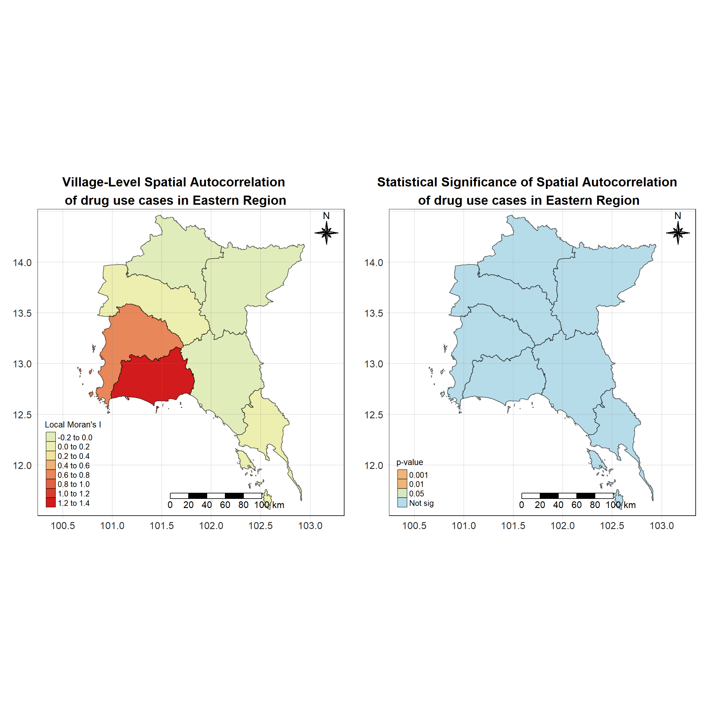

Southern Region

southern_local <- tm_shape(southern_lisa_2019)+
  tm_fill("ii", 
          palette = c("#e1ecbb","#f5f3a6", "#ec9a64","#de573e","#d21b1c"),
          title = "Local Moran's I",
          midpoint = NA) +
  tm_borders(col = "black", alpha = 0.6)+
  tm_layout(main.title = "Village-Level Spatial Autocorrelation \nof drug use cases in Southern Region",
            main.title.position = "center",
            main.title.size = 1.3,
            main.title.fontface = "bold",
            legend.title.size = 1,
            legend.text.size = 0.8,
            frame = TRUE) +
  tm_borders(alpha = 0.5) +
  tm_compass(type="8star", text.size = 1, size = 2, position=c("RIGHT", "TOP")) +
  tm_scale_bar(position=c("LEFT", "BOTTOM"), text.size=1) +
  tm_grid(labels.size = 1,alpha =0.2)

southern_sig <- tm_shape(southern_lisa_2019)+
  tm_fill("p_ii_sim", 
          palette = c("#d21b1c","#ec9a64","#f5f3a6","#c9e3d2","#b7dce9"),
          breaks = c(0, 0.001, 0.01, 0.05, 1),
          labels = c("0.001", "0.01", "0.05", "Not sig"), 
          title = "p-value",
          midpoint = NA) +
  tm_borders(col = "black", alpha = 0.6)+
  tm_layout(main.title = "Statistical Significance of Spatial Autocorrelation\n of drug use cases in Southern Region",
            main.title.position = "center",
            main.title.size = 1.3,
            main.title.fontface = "bold",
            legend.title.size = 1,
            legend.text.size = 0.8,
            frame = TRUE) +
  tm_borders(alpha = 0.5) +
  tm_compass(type="8star", text.size = 1, size = 2, position=c("RIGHT", "TOP")) +
  tm_scale_bar(position=c("LEFT", "BOTTOM"), text.size=1) +
  tm_grid(labels.size = 1,alpha =0.2)

tmap_arrange(southern_local,southern_sig, asp=1, ncol=2)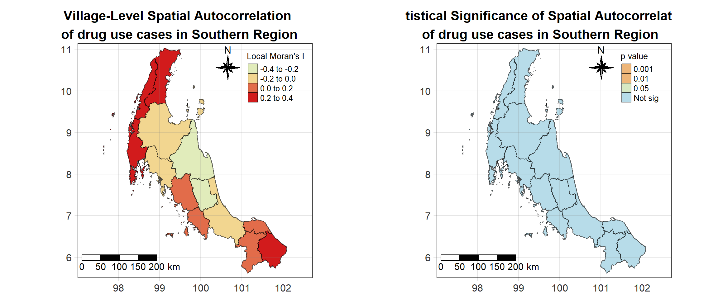

Analysis & Discussion

# Create the second map for northeastern_lisa_2019
northeastern_map <- tm_shape(northeastern_lisa_2019) +
  tm_polygons() +
  tm_borders(col = "black", alpha = 0.6) +
  tm_shape(northeastern_lisa_2019_sig) +
  tm_fill("mean", 
          palette = c("#b7dce9","#ec9a64","#e1ecbb", "#d21b1c"),
          title = "LISA class",
          midpoint = NA,
          legend.hist = TRUE, 
          legend.is.portrait = TRUE,
          legend.hist.z = 0.5) +
  tm_borders(col = "black", alpha = 0.6) +
  tm_layout(main.title = "2019 LISA plot of northeastern region",
            main.title.size = 0.8,
            legend.outside = TRUE)

# Create the first map for central_lisa_2019
central_map <- tm_shape(central_lisa_2019) +
  tm_polygons() +
  tm_borders(col = "black", alpha = 0.6) +
  tm_shape(central_lisa_2019_sig) +
  tm_fill("mean", 
          palette = c("#b7dce9","#ec9a64","#e1ecbb", "#d21b1c"),
          title = "LISA class",
          midpoint = NA,
          legend.hist = TRUE, 
          legend.is.portrait = TRUE,
          legend.hist.z = 0.5) +
  tm_borders(col = "black", alpha = 0.6) +
  tm_layout(main.title = "2019 LISA plot of central region",
            main.title.size = 0.8,
            legend.outside = TRUE)

# Arrange the two maps side by side
tmap_arrange(northeastern_map, central_map, asp=1, ncol=2)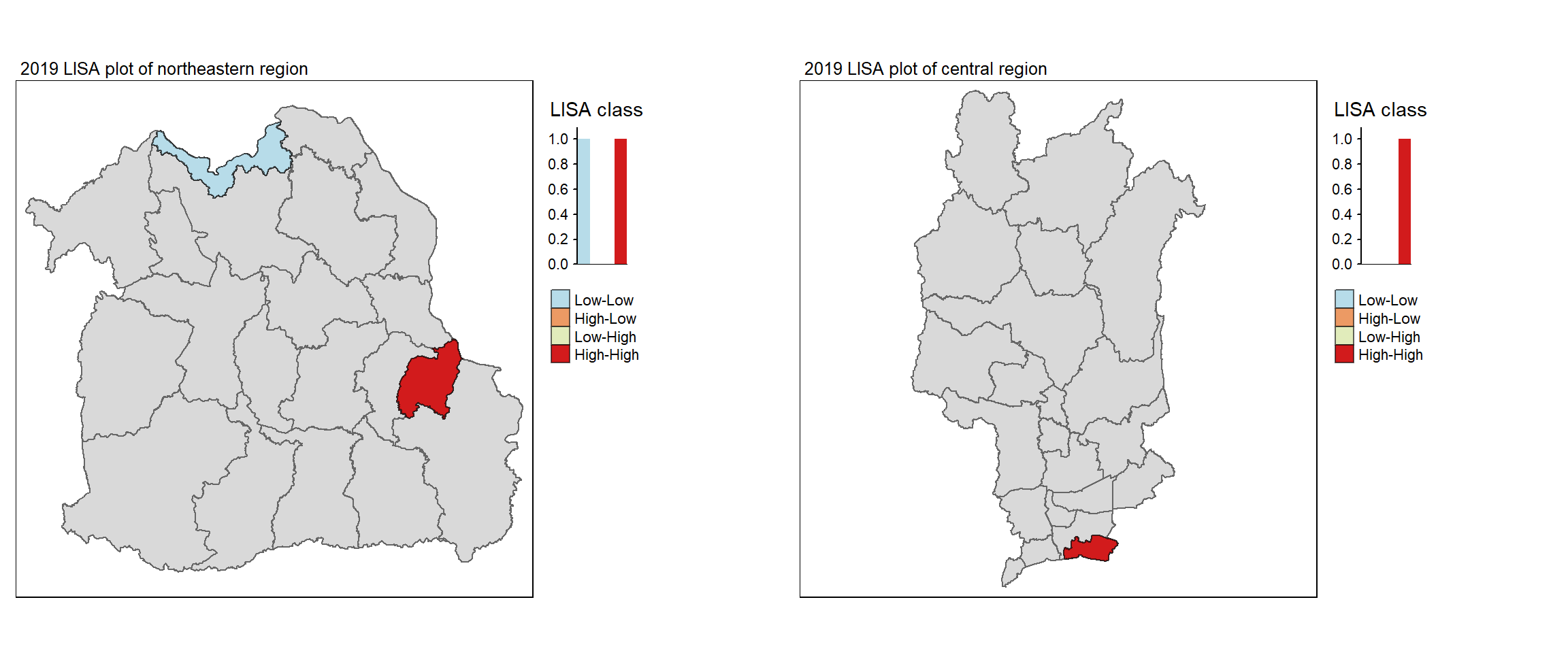

In 2019, the spatial autocorrelation patterns in the northeastern and central regions of Thailand present distinct shifts in drug use classifications compared to previous years.

In the Northeastern region (left plot), there is a notable concentration of High-High clusters in the southern part, indicating that provinces with high drug use rates are situated near other high-use provinces. Combined with the data from previous years, this suggests a persistence of drug-related issues in this area, requiring ongoing attention from policymakers and law enforcement. Additionally, some border provinces in the northern part of the region are classified as Low-Low, showing that these areas are characterized by low drug use rates surrounded by similarly low-use neighbors. This combination of clustering patterns highlights the complex landscape of drug use in the northeastern region, where areas of high intensity coexist with regions exhibiting stability in low usage.

In the Central region (right plot), we observe a significant presence of High-High clusters concentrated in the southern provinces, particularly in the province of Samut Prakan. This reinforces the trend of increased drug-related activities in this part of the region compared to the rest of the region as seen from the past 2 years.

Overall, both regions reveal a continued need for targeted interventions and policy adaptations to address the shifting patterns of drug use across Thailand’s northeastern and central regions. The persistence of high-use clusters in specific areas highlights the importance of focused resource allocation and strategic planning to combat drug-related challenges effectively.

Year 2020

northeastern_lisa_2020 <- lisa_2020 %>% filter(province_en %in% northeastern)
northern_lisa_2020 <- lisa_2020 %>% filter(province_en %in% northern)
western_lisa_2020 <- lisa_2020 %>% filter(province_en %in% western)
central_lisa_2020 <- lisa_2020 %>% filter(province_en %in% central)
eastern_lisa_2020 <- lisa_2020 %>% filter(province_en %in% eastern)
southern_lisa_2020 <- lisa_2020 %>% filter(province_en %in% southern)

northeastern_lisa_2020_sig <- lisa_2020_sig %>% filter(province_en %in% northeastern)
northern_lisa_2020_sig <- lisa_2020_sig %>% filter(province_en %in% northern)
western_lisa_2020_sig <- lisa_2020_sig %>% filter(province_en %in% western)
central_lisa_2020_sig <- lisa_2020_sig %>% filter(province_en %in% central)
eastern_lisa_2020_sig <- lisa_2020_sig %>% filter(province_en %in% eastern)
southern_lisa_2020_sig <- lisa_2020_sig %>% filter(province_en %in% southern)

Northeastern Region

northeastern_local <- tm_shape(northeastern_lisa_2020)+
  tm_fill("ii", 
          palette = c("#e1ecbb","#f5f3a6", "#ec9a64","#de573e","#d21b1c"),
          title = "Local Moran's I",
          midpoint = NA) +
  tm_borders(col = "black", alpha = 0.6)+
  tm_layout(main.title = "Village-Level Spatial Autocorrelation \nof drug use cases in Northeastern Region",
            main.title.position = "center",
            main.title.size = 1.3,
            main.title.fontface = "bold",
            legend.title.size = 1,
            legend.text.size = 0.8,
            frame = TRUE) +
  tm_borders(alpha = 0.5) +
  tm_compass(type="8star", text.size = 1, size = 2, position=c("RIGHT", "TOP")) +
  tm_scale_bar(position=c("LEFT", "BOTTOM"), text.size=1) +
  tm_grid(labels.size = 1,alpha =0.2)

northeastern_sig <- tm_shape(northeastern_lisa_2020)+
  tm_fill("p_ii_sim", 
          palette = c("#d21b1c","#ec9a64","#f5f3a6","#c9e3d2","#b7dce9"),
          breaks = c(0, 0.001, 0.01, 0.05, 1),
          labels = c("0.001", "0.01", "0.05", "Not sig"), 
          title = "p-value",
          midpoint = NA) +
  tm_borders(col = "black", alpha = 0.6)+
  tm_layout(main.title = "Statistical Significance of Spatial Autocorrelation\n of drug use cases in Northeastern Region",
            main.title.position = "center",
            main.title.size = 1.3,
            main.title.fontface = "bold",
            legend.title.size = 1,
            legend.text.size = 0.8,
            frame = TRUE) +
  tm_borders(alpha = 0.5) +
  tm_compass(type="8star", text.size = 1, size = 2, position=c("RIGHT", "TOP")) +
  tm_scale_bar(position=c("LEFT", "BOTTOM"), text.size=1) +
  tm_grid(labels.size = 1,alpha =0.2)

tmap_arrange(northeastern_local,northeastern_sig, asp=1, ncol=2)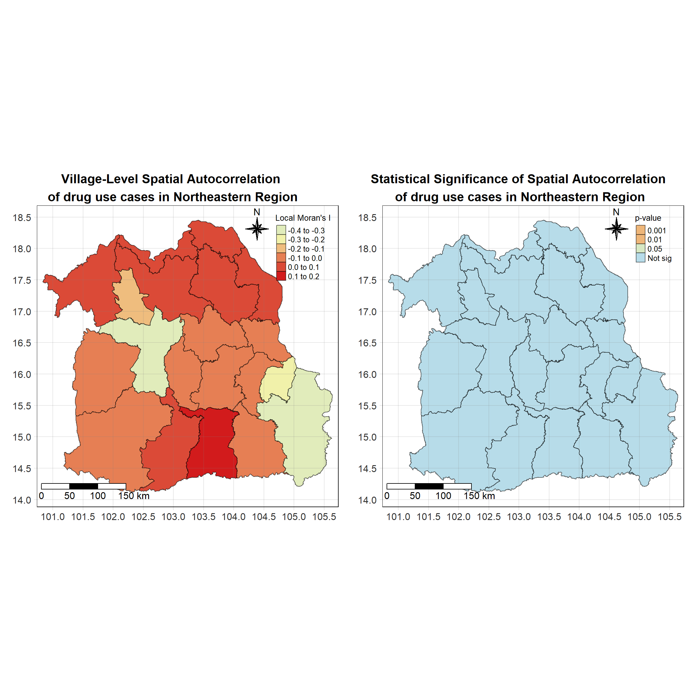

Northern Region

northern_local <- tm_shape(northern_lisa_2020)+
  tm_fill("ii", 
          palette = c("#e1ecbb","#f5f3a6", "#ec9a64","#de573e","#d21b1c"),
          title = "Local Moran's I",
          midpoint = NA) +
  tm_borders(col = "black", alpha = 0.6)+
  tm_layout(main.title = "Village-Level Spatial Autocorrelation \nof drug use cases in Northern Region",
            main.title.position = "center",
            main.title.size = 1.3,
            main.title.fontface = "bold",
            legend.title.size = 1,
            legend.text.size = 0.8,
            frame = TRUE) +
  tm_borders(alpha = 0.5) +
  tm_compass(type="8star", text.size = 1, size = 2, position=c("RIGHT", "TOP")) +
  tm_scale_bar(position=c("LEFT", "BOTTOM"), text.size=1) +
  tm_grid(labels.size = 1,alpha =0.2)

northern_sig <- tm_shape(northern_lisa_2020)+
  tm_fill("p_ii_sim", 
          palette = c("#d21b1c","#ec9a64","#f5f3a6","#c9e3d2","#b7dce9"),
          breaks = c(0, 0.001, 0.01, 0.05, 1),
          labels = c("0.001", "0.01", "0.05", "Not sig"), 
          title = "p-value",
          midpoint = NA) +
  tm_borders(col = "black", alpha = 0.6)+
  tm_layout(main.title = "Statistical Significance of Spatial Autocorrelation\n of drug use cases in North District",
            main.title.position = "center",
            main.title.size = 1.3,
            main.title.fontface = "bold",
            legend.title.size = 1,
            legend.text.size = 0.8,
            frame = TRUE) +
  tm_borders(alpha = 0.5) +
  tm_compass(type="8star", text.size = 1, size = 2, position=c("RIGHT", "TOP")) +
  tm_scale_bar(position=c("LEFT", "BOTTOM"), text.size=1) +
  tm_grid(labels.size = 1,alpha =0.2)

tmap_arrange(northern_local,northern_sig, asp=1, ncol=2)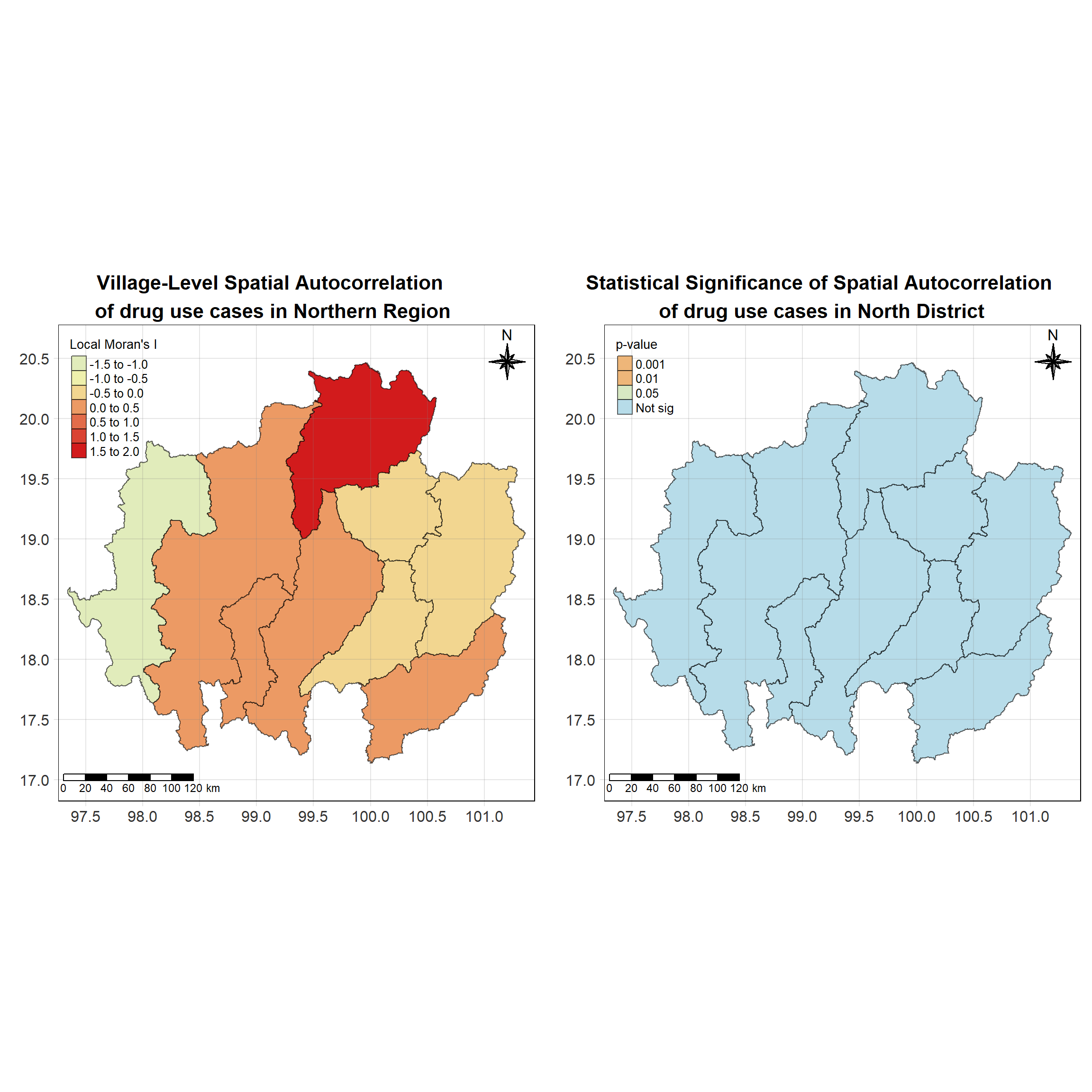

Western Region

western_local <- tm_shape(western_lisa_2020)+
  tm_fill("ii", 
          palette = c("#e1ecbb","#f5f3a6", "#ec9a64","#de573e","#d21b1c"),
          title = "Local Moran's I",
          midpoint = NA) +
  tm_borders(col = "black", alpha = 0.6)+
  tm_layout(main.title = "Village-Level Spatial Autocorrelation \nof drug use cases in North District",
            main.title.position = "center",
            main.title.size = 1.3,
            main.title.fontface = "bold",
            legend.title.size = 1,
            legend.text.size = 0.8,
            frame = TRUE) +
  tm_borders(alpha = 0.5) +
  tm_compass(type="8star", text.size = 1, size = 2, position=c("RIGHT", "TOP")) +
  tm_scale_bar(position=c("LEFT", "BOTTOM"), text.size=1) +
  tm_grid(labels.size = 1,alpha =0.2)

western_sig <- tm_shape(western_lisa_2020)+
  tm_fill("p_ii_sim", 
          palette = c("#d21b1c","#ec9a64","#f5f3a6","#c9e3d2","#b7dce9"),
          breaks = c(0, 0.001, 0.01, 0.05, 1),
          labels = c("0.001", "0.01", "0.05", "Not sig"), 
          title = "p-value",
          midpoint = NA) +
  tm_borders(col = "black", alpha = 0.6)+
  tm_layout(main.title = "Statistical Significance of Spatial Autocorrelation\n of drug use cases in North District",
            main.title.position = "center",
            main.title.size = 1.3,
            main.title.fontface = "bold",
            legend.title.size = 1,
            legend.text.size = 0.8,
            frame = TRUE) +
  tm_borders(alpha = 0.5) +
  tm_compass(type="8star", text.size = 1, size = 2, position=c("RIGHT", "TOP")) +
  tm_scale_bar(position=c("LEFT", "BOTTOM"), text.size=1) +
  tm_grid(labels.size = 1,alpha =0.2)

tmap_arrange(western_local,western_sig, asp=1, ncol=2)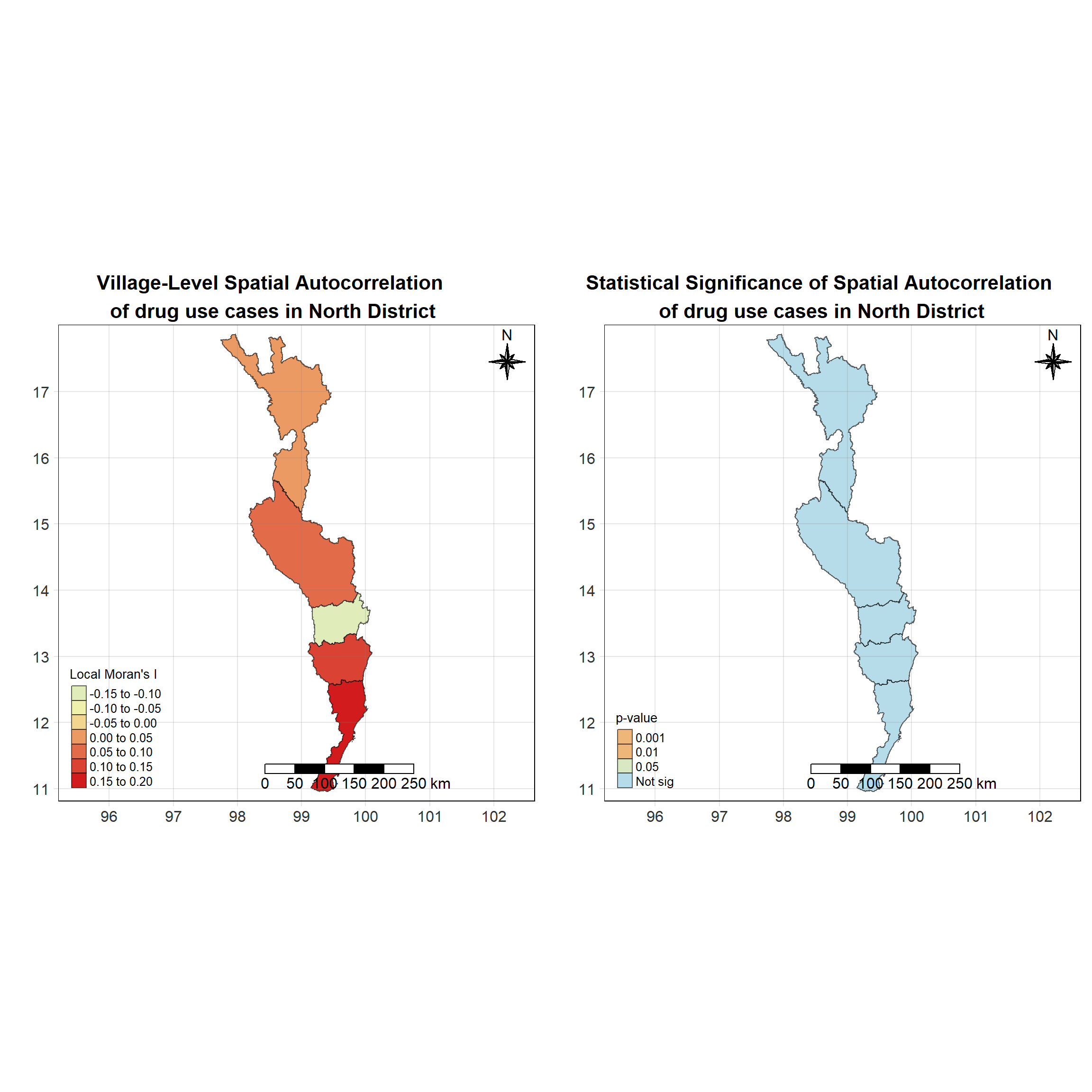

Central Region

central_local <- tm_shape(central_lisa_2020)+
  tm_fill("ii", 
          palette = c("#e1ecbb","#f5f3a6", "#ec9a64","#de573e","#d21b1c"),
          title = "Local Moran's I",
          midpoint = NA) +
  tm_borders(col = "black", alpha = 0.6)+
  tm_layout(main.title = "Village-Level Spatial Autocorrelation \nof drug use cases in North District",
            main.title.position = "center",
            main.title.size = 1.3,
            main.title.fontface = "bold",
            legend.title.size = 1,
            legend.text.size = 0.8,
            frame = TRUE) +
  tm_borders(alpha = 0.5) +
  tm_compass(type="8star", text.size = 1, size = 2, position=c("RIGHT", "TOP")) +
  tm_scale_bar(position=c("LEFT", "BOTTOM"), text.size=1) +
  tm_grid(labels.size = 1,alpha =0.2)

central_sig <- tm_shape(central_lisa_2020)+
  tm_fill("p_ii_sim", 
          palette = c("#d21b1c","#ec9a64","#f5f3a6","#c9e3d2","#b7dce9"),
          breaks = c(0, 0.001, 0.01, 0.05, 1),
          labels = c("0.001", "0.01", "0.05", "Not sig"), 
          title = "p-value",
          midpoint = NA) +
  tm_borders(col = "black", alpha = 0.6)+
  tm_layout(main.title = "Statistical Significance of Spatial Autocorrelation\n of drug use cases in North District",
            main.title.position = "center",
            main.title.size = 1.3,
            main.title.fontface = "bold",
            legend.title.size = 1,
            legend.text.size = 0.8,
            frame = TRUE) +
  tm_borders(alpha = 0.5) +
  tm_compass(type="8star", text.size = 1, size = 2, position=c("RIGHT", "TOP")) +
  tm_scale_bar(position=c("LEFT", "BOTTOM"), text.size=1) +
  tm_grid(labels.size = 1,alpha =0.2)

tmap_arrange(central_local,central_sig, asp=1, ncol=2)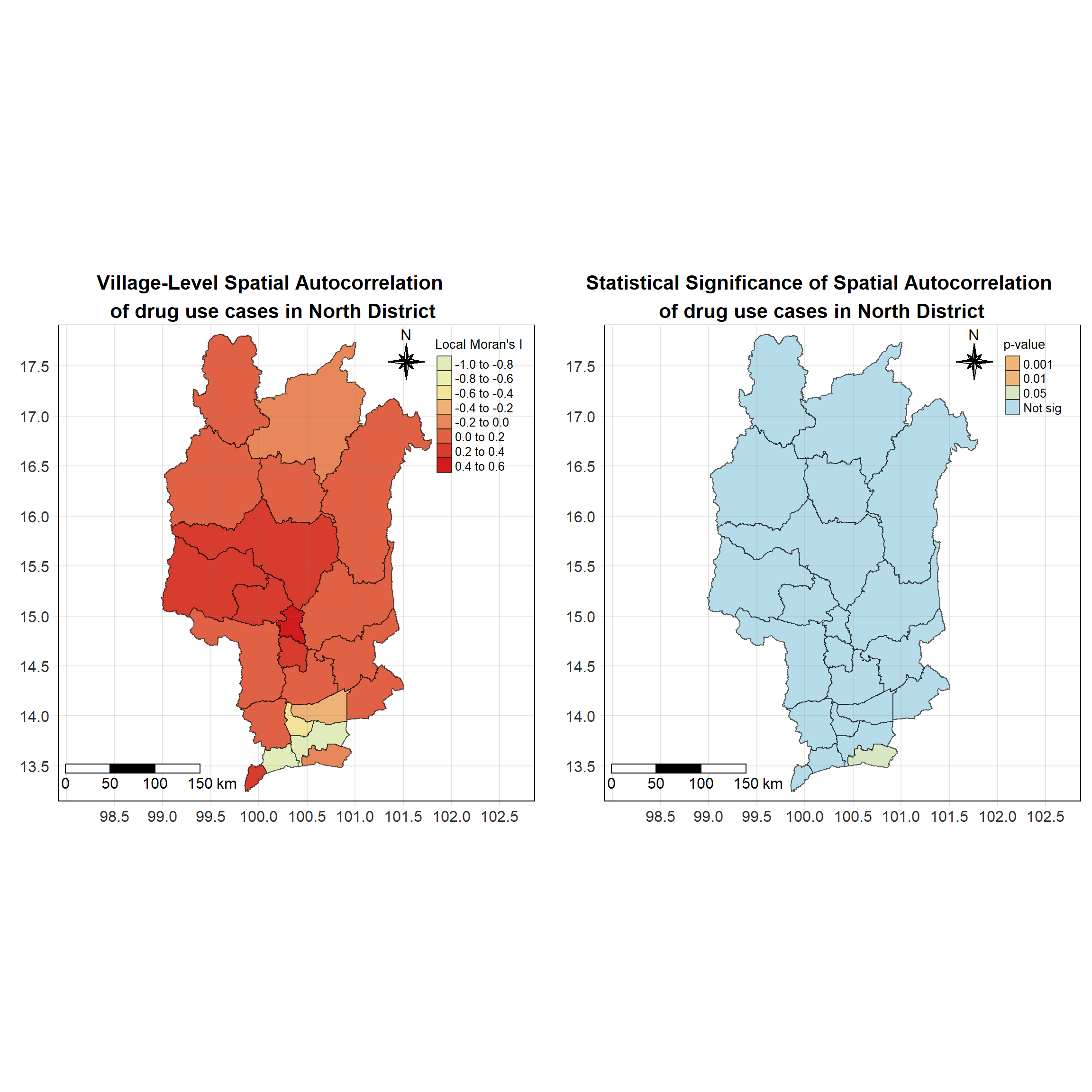

Eastern Region

eastern_local <- tm_shape(eastern_lisa_2020)+
  tm_fill("ii", 
          palette = c("#e1ecbb","#f5f3a6", "#ec9a64","#de573e","#d21b1c"),
          title = "Local Moran's I",
          midpoint = NA) +
  tm_borders(col = "black", alpha = 0.6)+
  tm_layout(main.title = "Village-Level Spatial Autocorrelation \nof drug use cases in North District",
            main.title.position = "center",
            main.title.size = 1.3,
            main.title.fontface = "bold",
            legend.title.size = 1,
            legend.text.size = 0.8,
            frame = TRUE) +
  tm_borders(alpha = 0.5) +
  tm_compass(type="8star", text.size = 1, size = 2, position=c("RIGHT", "TOP")) +
  tm_scale_bar(position=c("LEFT", "BOTTOM"), text.size=1) +
  tm_grid(labels.size = 1,alpha =0.2)

eastern_sig <- tm_shape(eastern_lisa_2020)+
  tm_fill("p_ii_sim", 
          palette = c("#d21b1c","#ec9a64","#f5f3a6","#c9e3d2","#b7dce9"),
          breaks = c(0, 0.001, 0.01, 0.05, 1),
          labels = c("0.001", "0.01", "0.05", "Not sig"), 
          title = "p-value",
          midpoint = NA) +
  tm_borders(col = "black", alpha = 0.6)+
  tm_layout(main.title = "Statistical Significance of Spatial Autocorrelation\n of drug use cases in North District",
            main.title.position = "center",
            main.title.size = 1.3,
            main.title.fontface = "bold",
            legend.title.size = 1,
            legend.text.size = 0.8,
            frame = TRUE) +
  tm_borders(alpha = 0.5) +
  tm_compass(type="8star", text.size = 1, size = 2, position=c("RIGHT", "TOP")) +
  tm_scale_bar(position=c("LEFT", "BOTTOM"), text.size=1) +
  tm_grid(labels.size = 1,alpha =0.2)

tmap_arrange(eastern_local,eastern_sig, asp=1, ncol=2)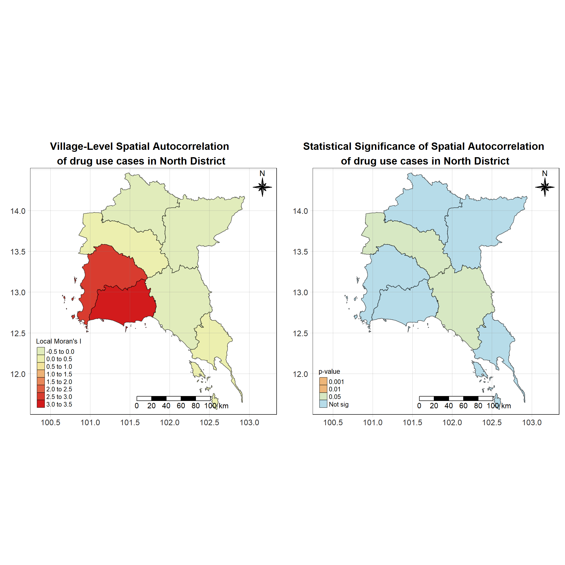

Southern Region

southern_local <- tm_shape(southern_lisa_2020)+
  tm_fill("ii", 
          palette = c("#e1ecbb","#f5f3a6", "#ec9a64","#de573e","#d21b1c"),
          title = "Local Moran's I",
          midpoint = NA) +
  tm_borders(col = "black", alpha = 0.6)+
  tm_layout(main.title = "Village-Level Spatial Autocorrelation \nof drug use cases in North District",
            main.title.position = "center",
            main.title.size = 1.3,
            main.title.fontface = "bold",
            legend.title.size = 1,
            legend.text.size = 0.8,
            frame = TRUE) +
  tm_borders(alpha = 0.5) +
  tm_compass(type="8star", text.size = 1, size = 2, position=c("RIGHT", "TOP")) +
  tm_scale_bar(position=c("LEFT", "BOTTOM"), text.size=1) +
  tm_grid(labels.size = 1,alpha =0.2)

southern_sig <- tm_shape(southern_lisa_2020)+
  tm_fill("p_ii_sim", 
          palette = c("#d21b1c","#ec9a64","#f5f3a6","#c9e3d2","#b7dce9"),
          breaks = c(0, 0.001, 0.01, 0.05, 1),
          labels = c("0.001", "0.01", "0.05", "Not sig"), 
          title = "p-value",
          midpoint = NA) +
  tm_borders(col = "black", alpha = 0.6)+
  tm_layout(main.title = "Statistical Significance of Spatial Autocorrelation\n of drug use cases in North District",
            main.title.position = "center",
            main.title.size = 1.3,
            main.title.fontface = "bold",
            legend.title.size = 1,
            legend.text.size = 0.8,
            frame = TRUE) +
  tm_borders(alpha = 0.5) +
  tm_compass(type="8star", text.size = 1, size = 2, position=c("RIGHT", "TOP")) +
  tm_scale_bar(position=c("LEFT", "BOTTOM"), text.size=1) +
  tm_grid(labels.size = 1,alpha =0.2)

tmap_arrange(southern_local,southern_sig, asp=1, ncol=2)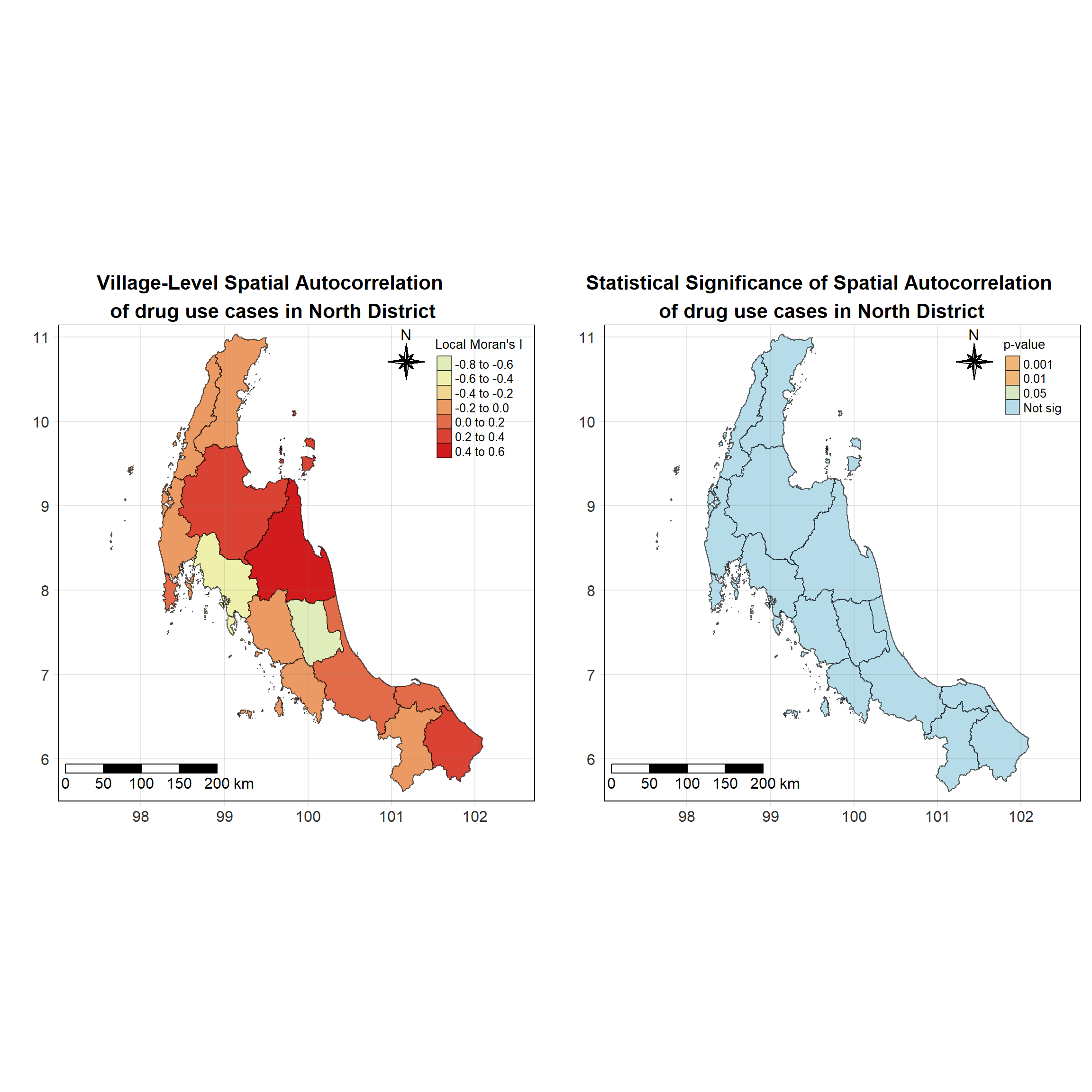

Analysis & Discussion

# Create the first map for central_lisa_2020
central_map <- tm_shape(central_lisa_2020) +
  tm_polygons() +
  tm_borders(col = "black", alpha = 0.6) +
  tm_shape(central_lisa_2020_sig) +
  tm_fill("mean", 
          palette = c("#b7dce9","#ec9a64","#e1ecbb", "#d21b1c"),
          title = "LISA class",
          midpoint = NA,
          legend.hist = TRUE, 
          legend.is.portrait = TRUE,
          legend.hist.z = 0.5) +
  tm_borders(col = "black", alpha = 0.6) +
  tm_layout(main.title = "2020 LISA plot of central region",
            main.title.size = 0.8,
            legend.outside = TRUE)

# Create the second map for eastern_lisa_2020
eastern_map <- tm_shape(eastern_lisa_2020) +
  tm_polygons() +
  tm_borders(col = "black", alpha = 0.6) +
  tm_shape(eastern_lisa_2020_sig) +
  tm_fill("mean", 
          palette = c("#b7dce9","#ec9a64","#e1ecbb", "#d21b1c"),
          title = "LISA class",
          midpoint = NA,
          legend.hist = TRUE, 
          legend.is.portrait = TRUE,
          legend.hist.z = 0.5) +
  tm_borders(col = "black", alpha = 0.6) +
  tm_layout(main.title = "2020 LISA plot of eastern region",
            main.title.size = 0.8,
            legend.outside = TRUE)

# Arrange the two maps side by side
tmap_arrange(central_map, eastern_map, asp=1, ncol=2)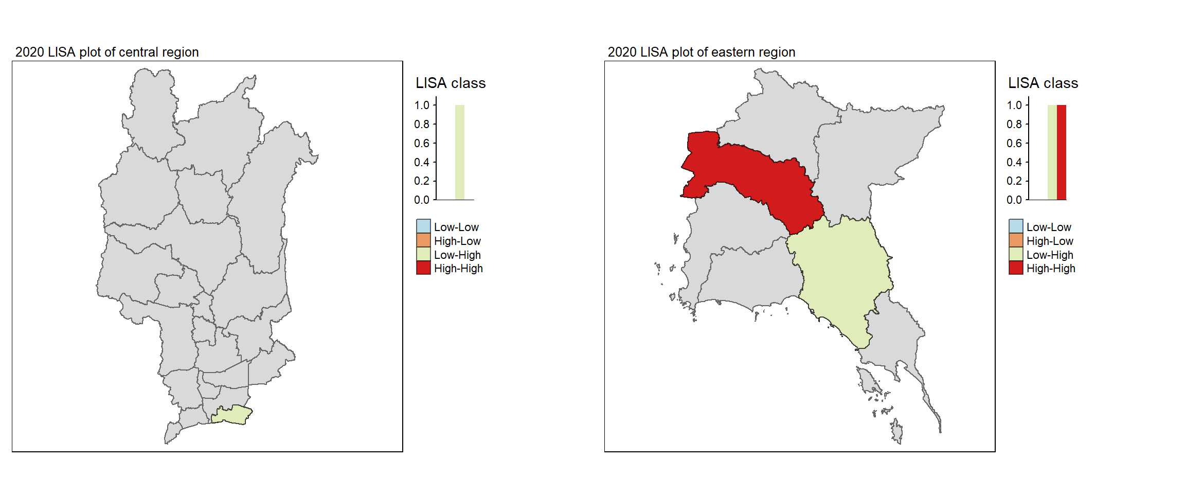

In 2020, the spatial autocorrelation patterns in the eastern and central regions of Thailand present distinct shifts in drug use classifications compared to previous years.

In the Central region (left plot), there is a notable concentration of Low-High clusters in the southern part, indicating that provinces with high drug use rates are situated near other high-use provinces. Combined with the data from previous years, this suggests a persistence of drug-related issues in this area, requiring ongoing attention from policymakers and law enforcement.

In the Eastern region (right plot), we observe some border provinces in the northern part of the region are classified as Low-High, showing that these areas are characterized by low drug use rates surrounded by high-use neighbors. It is noteworthy that the area is also at the eastern border, similar to those clusters in the previous years. Additionally, a significant presence of High-High clusters concentrated in the western provinces, particularly in the province of Chachoengsao. This cluster is neigbhouring the Low-High cluster of Central region, connecting the 2020 highlighted clusters together in both regions.

Overall, both regions reveal a continued need for targeted interventions and policy adaptations to address the shifting patterns of drug use across Thailand’s regions. The persistence of high-use clusters in the eastern border provinces and central region specifically highlights the importance of focused resource allocation and strategic planning to combat drug-related challenges effectively.

Year 2021

northeastern_lisa_2021 <- lisa_2021 %>% filter(province_en %in% northeastern)
northern_lisa_2021 <- lisa_2021 %>% filter(province_en %in% northern)
western_lisa_2021 <- lisa_2021 %>% filter(province_en %in% western)
central_lisa_2021 <- lisa_2021 %>% filter(province_en %in% central)
eastern_lisa_2021 <- lisa_2021 %>% filter(province_en %in% eastern)
southern_lisa_2021 <- lisa_2021 %>% filter(province_en %in% southern)

northeastern_lisa_2021_sig <- lisa_2021_sig %>% filter(province_en %in% northeastern)
northern_lisa_2021_sig <- lisa_2021_sig %>% filter(province_en %in% northern)
western_lisa_2021_sig <- lisa_2021_sig %>% filter(province_en %in% western)
central_lisa_2021_sig <- lisa_2021_sig %>% filter(province_en %in% central)
eastern_lisa_2021_sig <- lisa_2021_sig %>% filter(province_en %in% eastern)
southern_lisa_2021_sig <- lisa_2021_sig %>% filter(province_en %in% southern)

Northeastern Region

northeastern_local <- tm_shape(northeastern_lisa_2021)+
  tm_fill("ii", 
          palette = c("#e1ecbb","#f5f3a6", "#ec9a64","#de573e","#d21b1c"),
          title = "Local Moran's I",
          midpoint = NA) +
  tm_borders(col = "black", alpha = 0.6)+
  tm_layout(main.title = "Village-Level Spatial Autocorrelation \nof drug use cases in North District",
            main.title.position = "center",
            main.title.size = 1.3,
            main.title.fontface = "bold",
            legend.title.size = 1,
            legend.text.size = 0.8,
            frame = TRUE) +
  tm_borders(alpha = 0.5) +
  tm_compass(type="8star", text.size = 1, size = 2, position=c("RIGHT", "TOP")) +
  tm_scale_bar(position=c("LEFT", "BOTTOM"), text.size=1) +
  tm_grid(labels.size = 1,alpha =0.2)

northeastern_sig <- tm_shape(northeastern_lisa_2021)+
  tm_fill("p_ii_sim", 
          palette = c("#d21b1c","#ec9a64","#f5f3a6","#c9e3d2","#b7dce9"),
          breaks = c(0, 0.001, 0.01, 0.05, 1),
          labels = c("0.001", "0.01", "0.05", "Not sig"), 
          title = "p-value",
          midpoint = NA) +
  tm_borders(col = "black", alpha = 0.6)+
  tm_layout(main.title = "Statistical Significance of Spatial Autocorrelation\n of drug use cases in North District",
            main.title.position = "center",
            main.title.size = 1.3,
            main.title.fontface = "bold",
            legend.title.size = 1,
            legend.text.size = 0.8,
            frame = TRUE) +
  tm_borders(alpha = 0.5) +
  tm_compass(type="8star", text.size = 1, size = 2, position=c("RIGHT", "TOP")) +
  tm_scale_bar(position=c("LEFT", "BOTTOM"), text.size=1) +
  tm_grid(labels.size = 1,alpha =0.2)

tmap_arrange(northeastern_local,northeastern_sig, asp=1, ncol=2)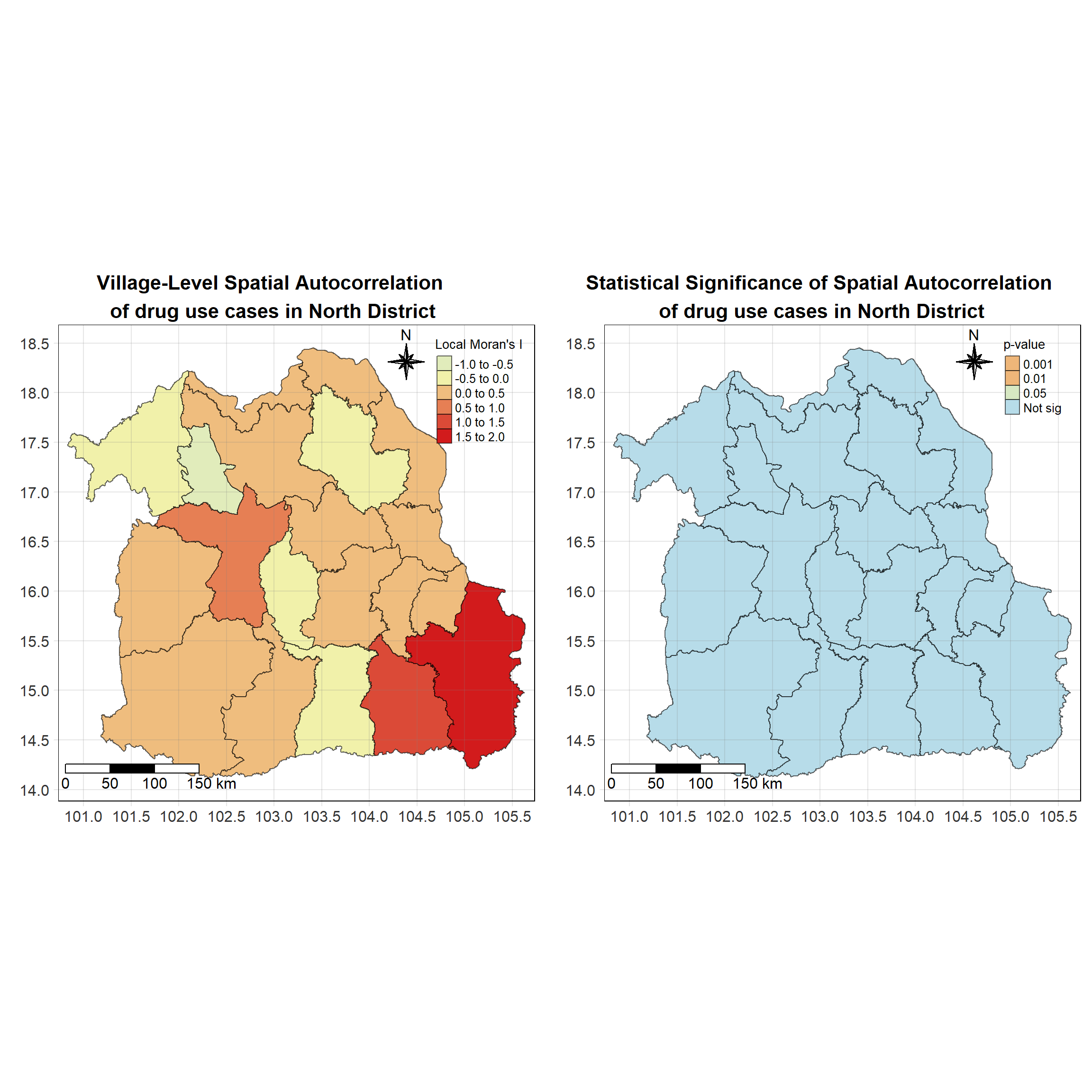

Northern Region

northern_local <- tm_shape(northern_lisa_2021)+
  tm_fill("ii", 
          palette = c("#e1ecbb","#f5f3a6", "#ec9a64","#de573e","#d21b1c"),
          title = "Local Moran's I",
          midpoint = NA) +
  tm_borders(col = "black", alpha = 0.6)+
  tm_layout(main.title = "Village-Level Spatial Autocorrelation \nof drug use cases in North District",
            main.title.position = "center",
            main.title.size = 1.3,
            main.title.fontface = "bold",
            legend.title.size = 1,
            legend.text.size = 0.8,
            frame = TRUE) +
  tm_borders(alpha = 0.5) +
  tm_compass(type="8star", text.size = 1, size = 2, position=c("RIGHT", "TOP")) +
  tm_scale_bar(position=c("LEFT", "BOTTOM"), text.size=1) +
  tm_grid(labels.size = 1,alpha =0.2)

northern_sig <- tm_shape(northern_lisa_2021)+
  tm_fill("p_ii_sim", 
          palette = c("#d21b1c","#ec9a64","#f5f3a6","#c9e3d2","#b7dce9"),
          breaks = c(0, 0.001, 0.01, 0.05, 1),
          labels = c("0.001", "0.01", "0.05", "Not sig"), 
          title = "p-value",
          midpoint = NA) +
  tm_borders(col = "black", alpha = 0.6)+
  tm_layout(main.title = "Statistical Significance of Spatial Autocorrelation\n of drug use cases in North District",
            main.title.position = "center",
            main.title.size = 1.3,
            main.title.fontface = "bold",
            legend.title.size = 1,
            legend.text.size = 0.8,
            frame = TRUE) +
  tm_borders(alpha = 0.5) +
  tm_compass(type="8star", text.size = 1, size = 2, position=c("RIGHT", "TOP")) +
  tm_scale_bar(position=c("LEFT", "BOTTOM"), text.size=1) +
  tm_grid(labels.size = 1,alpha =0.2)

tmap_arrange(northern_local,northern_sig, asp=1, ncol=2)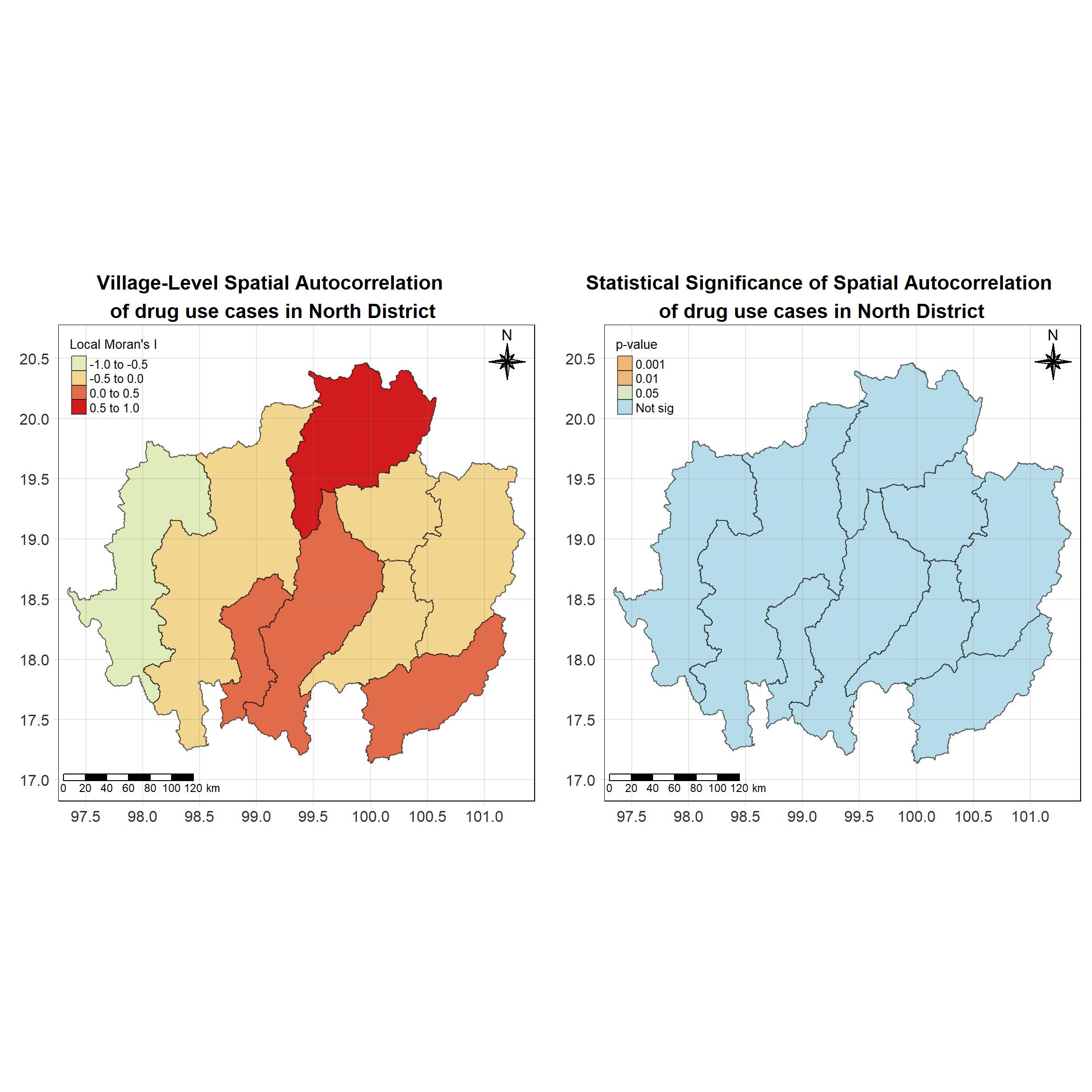

Western Region

western_local <- tm_shape(western_lisa_2021)+
  tm_fill("ii", 
          palette = c("#e1ecbb","#f5f3a6", "#ec9a64","#de573e","#d21b1c"),
          title = "Local Moran's I",
          midpoint = NA) +
  tm_borders(col = "black", alpha = 0.6)+
  tm_layout(main.title = "Village-Level Spatial Autocorrelation \nof drug use cases in North District",
            main.title.position = "center",
            main.title.size = 1.3,
            main.title.fontface = "bold",
            legend.title.size = 1,
            legend.text.size = 0.8,
            frame = TRUE) +
  tm_borders(alpha = 0.5) +
  tm_compass(type="8star", text.size = 1, size = 2, position=c("RIGHT", "TOP")) +
  tm_scale_bar(position=c("LEFT", "BOTTOM"), text.size=1) +
  tm_grid(labels.size = 1,alpha =0.2)

western_sig <- tm_shape(western_lisa_2021)+
  tm_fill("p_ii_sim", 
          palette = c("#d21b1c","#ec9a64","#f5f3a6","#c9e3d2","#b7dce9"),
          breaks = c(0, 0.001, 0.01, 0.05, 1),
          labels = c("0.001", "0.01", "0.05", "Not sig"), 
          title = "p-value",
          midpoint = NA) +
  tm_borders(col = "black", alpha = 0.6)+
  tm_layout(main.title = "Statistical Significance of Spatial Autocorrelation\n of drug use cases in North District",
            main.title.position = "center",
            main.title.size = 1.3,
            main.title.fontface = "bold",
            legend.title.size = 1,
            legend.text.size = 0.8,
            frame = TRUE) +
  tm_borders(alpha = 0.5) +
  tm_compass(type="8star", text.size = 1, size = 2, position=c("RIGHT", "TOP")) +
  tm_scale_bar(position=c("LEFT", "BOTTOM"), text.size=1) +
  tm_grid(labels.size = 1,alpha =0.2)

tmap_arrange(western_local,western_sig, asp=1, ncol=2)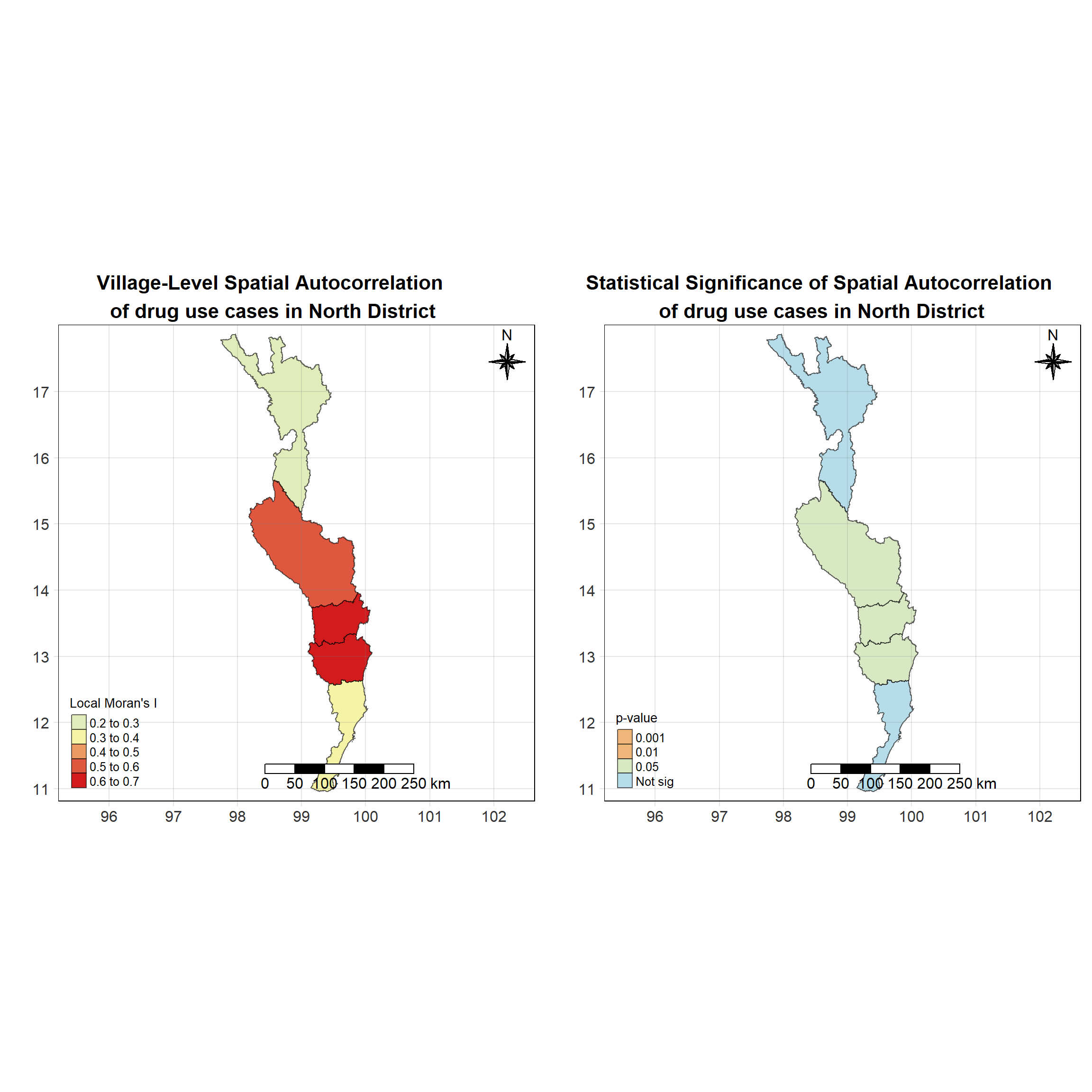

Central Region

central_local <- tm_shape(central_lisa_2021)+
  tm_fill("ii", 
          palette = c("#e1ecbb","#f5f3a6", "#ec9a64","#de573e","#d21b1c"),
          title = "Local Moran's I",
          midpoint = NA) +
  tm_borders(col = "black", alpha = 0.6)+
  tm_layout(main.title = "Village-Level Spatial Autocorrelation \nof drug use cases in North District",
            main.title.position = "center",
            main.title.size = 1.3,
            main.title.fontface = "bold",
            legend.title.size = 1,
            legend.text.size = 0.8,
            frame = TRUE) +
  tm_borders(alpha = 0.5) +
  tm_compass(type="8star", text.size = 1, size = 2, position=c("RIGHT", "TOP")) +
  tm_scale_bar(position=c("LEFT", "BOTTOM"), text.size=1) +
  tm_grid(labels.size = 1,alpha =0.2)

central_sig <- tm_shape(central_lisa_2021)+
  tm_fill("p_ii_sim", 
          palette = c("#d21b1c","#ec9a64","#f5f3a6","#c9e3d2","#b7dce9"),
          breaks = c(0, 0.001, 0.01, 0.05, 1),
          labels = c("0.001", "0.01", "0.05", "Not sig"), 
          title = "p-value",
          midpoint = NA) +
  tm_borders(col = "black", alpha = 0.6)+
  tm_layout(main.title = "Statistical Significance of Spatial Autocorrelation\n of drug use cases in North District",
            main.title.position = "center",
            main.title.size = 1.3,
            main.title.fontface = "bold",
            legend.title.size = 1,
            legend.text.size = 0.8,
            frame = TRUE) +
  tm_borders(alpha = 0.5) +
  tm_compass(type="8star", text.size = 1, size = 2, position=c("RIGHT", "TOP")) +
  tm_scale_bar(position=c("LEFT", "BOTTOM"), text.size=1) +
  tm_grid(labels.size = 1,alpha =0.2)

tmap_arrange(central_local,central_sig, asp=1, ncol=2)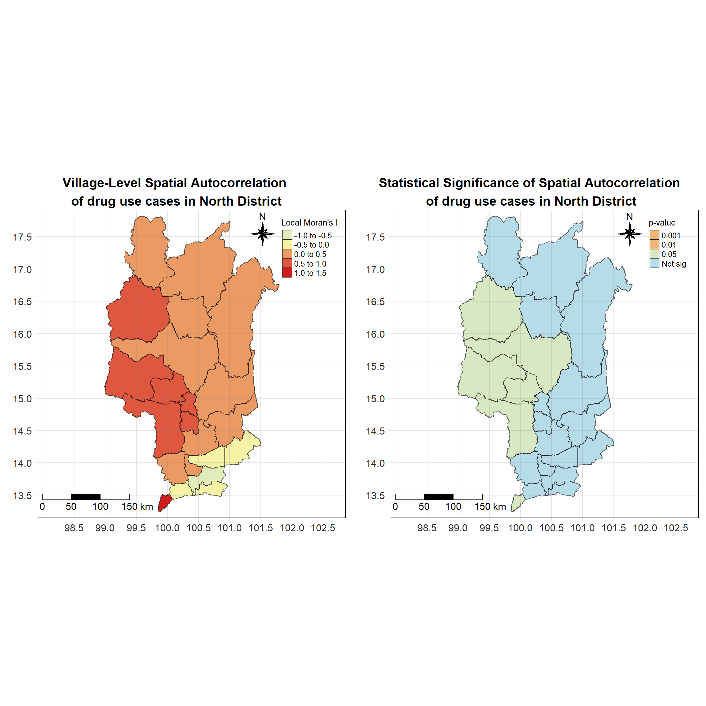

Eastern Region

eastern_local <- tm_shape(eastern_lisa_2021)+
  tm_fill("ii", 
          palette = c("#e1ecbb","#f5f3a6", "#ec9a64","#de573e","#d21b1c"),
          title = "Local Moran's I",
          midpoint = NA) +
  tm_borders(col = "black", alpha = 0.6)+
  tm_layout(main.title = "Village-Level Spatial Autocorrelation \nof drug use cases in North District",
            main.title.position = "center",
            main.title.size = 1.3,
            main.title.fontface = "bold",
            legend.title.size = 1,
            legend.text.size = 0.8,
            frame = TRUE) +
  tm_borders(alpha = 0.5) +
  tm_compass(type="8star", text.size = 1, size = 2, position=c("RIGHT", "TOP")) +
  tm_scale_bar(position=c("LEFT", "BOTTOM"), text.size=1) +
  tm_grid(labels.size = 1,alpha =0.2)

eastern_sig <- tm_shape(eastern_lisa_2021)+
  tm_fill("p_ii_sim", 
          palette = c("#d21b1c","#ec9a64","#f5f3a6","#c9e3d2","#b7dce9"),
          breaks = c(0, 0.001, 0.01, 0.05, 1),
          labels = c("0.001", "0.01", "0.05", "Not sig"), 
          title = "p-value",
          midpoint = NA) +
  tm_borders(col = "black", alpha = 0.6)+
  tm_layout(main.title = "Statistical Significance of Spatial Autocorrelation\n of drug use cases in North District",
            main.title.position = "center",
            main.title.size = 1.3,
            main.title.fontface = "bold",
            legend.title.size = 1,
            legend.text.size = 0.8,
            frame = TRUE) +
  tm_borders(alpha = 0.5) +
  tm_compass(type="8star", text.size = 1, size = 2, position=c("RIGHT", "TOP")) +
  tm_scale_bar(position=c("LEFT", "BOTTOM"), text.size=1) +
  tm_grid(labels.size = 1,alpha =0.2)

tmap_arrange(eastern_local,eastern_sig, asp=1, ncol=2)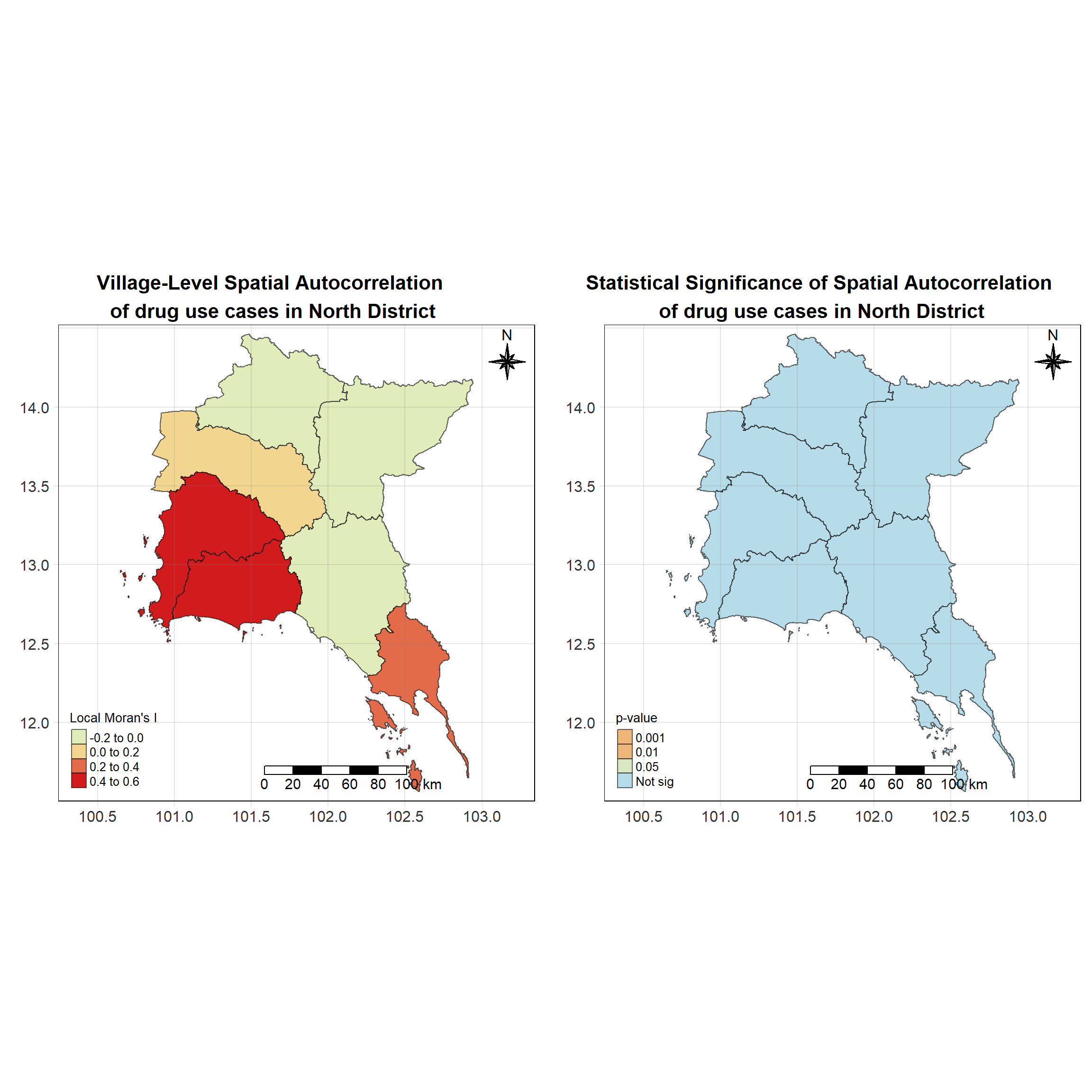

Southern Region

southern_local <- tm_shape(southern_lisa_2021)+
  tm_fill("ii", 
          palette = c("#e1ecbb","#f5f3a6", "#ec9a64","#de573e","#d21b1c"),
          title = "Local Moran's I",
          midpoint = NA) +
  tm_borders(col = "black", alpha = 0.6)+
  tm_layout(main.title = "Village-Level Spatial Autocorrelation \nof drug use cases in North District",
            main.title.position = "center",
            main.title.size = 1.3,
            main.title.fontface = "bold",
            legend.title.size = 1,
            legend.text.size = 0.8,
            frame = TRUE) +
  tm_borders(alpha = 0.5) +
  tm_compass(type="8star", text.size = 1, size = 2, position=c("RIGHT", "TOP")) +
  tm_scale_bar(position=c("LEFT", "BOTTOM"), text.size=1) +
  tm_grid(labels.size = 1,alpha =0.2)

southern_sig <- tm_shape(southern_lisa_2021)+
  tm_fill("p_ii_sim", 
          palette = c("#d21b1c","#ec9a64","#f5f3a6","#c9e3d2","#b7dce9"),
          breaks = c(0, 0.001, 0.01, 0.05, 1),
          labels = c("0.001", "0.01", "0.05", "Not sig"), 
          title = "p-value",
          midpoint = NA) +
  tm_borders(col = "black", alpha = 0.6)+
  tm_layout(main.title = "Statistical Significance of Spatial Autocorrelation\n of drug use cases in North District",
            main.title.position = "center",
            main.title.size = 1.3,
            main.title.fontface = "bold",
            legend.title.size = 1,
            legend.text.size = 0.8,
            frame = TRUE) +
  tm_borders(alpha = 0.5) +
  tm_compass(type="8star", text.size = 1, size = 2, position=c("RIGHT", "TOP")) +
  tm_scale_bar(position=c("LEFT", "BOTTOM"), text.size=1) +
  tm_grid(labels.size = 1,alpha =0.2)

tmap_arrange(southern_local,southern_sig, asp=1, ncol=2)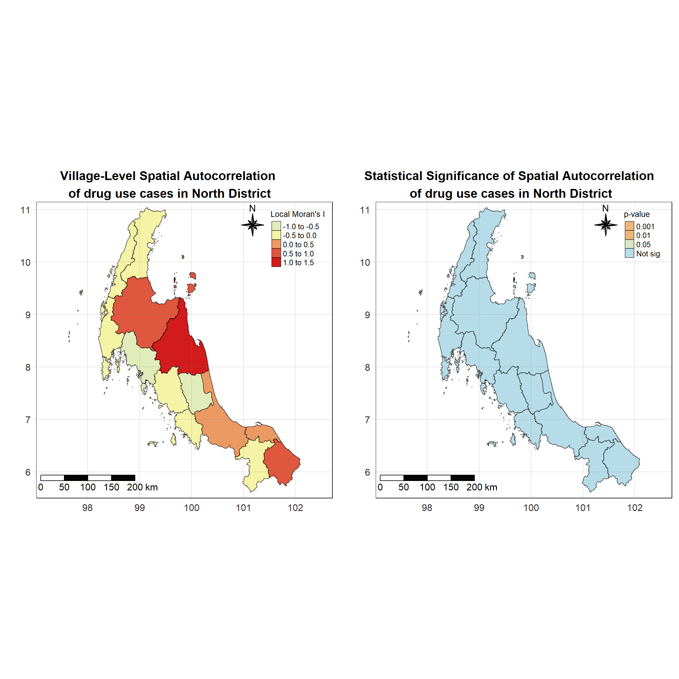

Analysis & Discussion

# Create the second map for western_lisa_2021
western_map <- tm_shape(western_lisa_2021) +
  tm_polygons() +
  tm_borders(col = "black", alpha = 0.6) +
  tm_shape(western_lisa_2021_sig) +
  tm_fill("mean", 
          palette = c("#b7dce9","#ec9a64","#e1ecbb", "#d21b1c"),
          title = "LISA class",
          midpoint = NA,
          legend.hist = TRUE, 
          legend.is.portrait = TRUE,
          legend.hist.z = 0.5) +
  tm_borders(col = "black", alpha = 0.6) +
  tm_layout(main.title = "2021 LISA plot of western region",
            main.title.size = 0.8,
            legend.outside = TRUE)

# Create the first map for central_lisa_2021
central_map <- tm_shape(central_lisa_2021) +
  tm_polygons() +
  tm_borders(col = "black", alpha = 0.6) +
  tm_shape(central_lisa_2021_sig) +
  tm_fill("mean", 
          palette = c("#b7dce9","#ec9a64","#e1ecbb", "#d21b1c"),
          title = "LISA class",
          midpoint = NA,
          legend.hist = TRUE, 
          legend.is.portrait = TRUE,
          legend.hist.z = 0.5) +
  tm_borders(col = "black", alpha = 0.6) +
  tm_layout(main.title = "2021 LISA plot of central region",
            main.title.size = 0.8,
            legend.outside = TRUE)

# Arrange the two maps side by side
tmap_arrange(western_map, central_map, asp=1, ncol=2)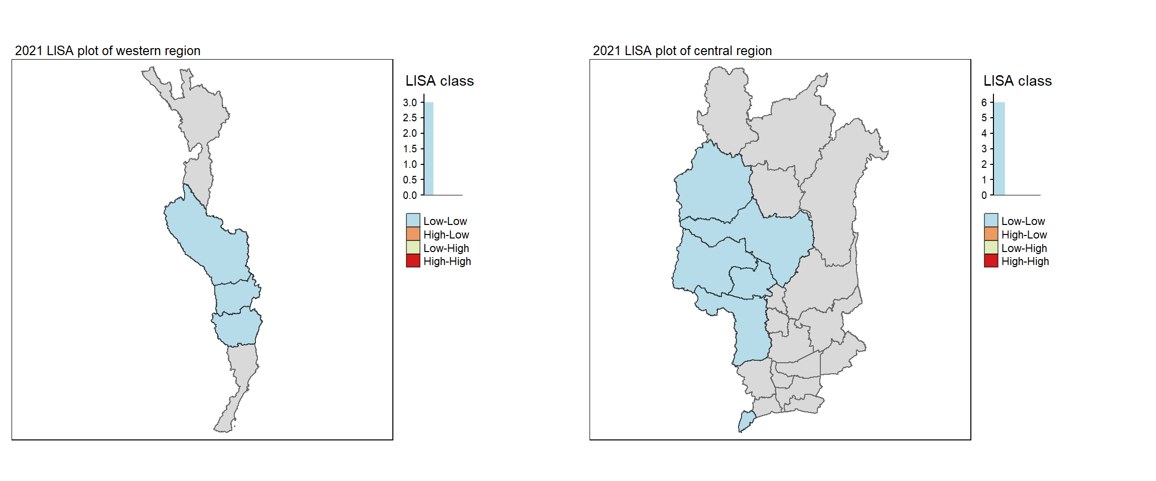

In 2021, the spatial autocorrelation patterns in the western and central regions of Thailand present distinct shifts in drug use classifications compared to previous years.

In the Western region (left plot), there is a notable concentration of Low-Low clusters in the central part. These clusters indicate that these provinces and their neighbors experience consistently lower drug-related cases compared to the rest of the region.

In the Central region (right plot), we observe a significant presence of Low-Low clusters concentrated in the western and southern provinces. These cluster is neigbhouring the Low-Low cluster of Western region, connecting the 2021 highlighted clusters together in both regions. This shows that this areas are characterized by low drug use rates surrounded by low-use neighbors.

Overall, the plots highlight a significant presence of Low-Low clusters in both the Western and Central regions, suggesting that several provinces in these areas have lower-than-average drug-related cases compared to their neighbors. The patterns are consistent across multiple neighbouring provinces, indicating potential coldspots that may benefit from maintaining existing preventative measures. Additionally, the absence of High-High clusters in all regions for 2021 implies that there were no significant hotspots for drug abuse activity, indicating either a reduction in drug-related cases or a more uniform distribution across these regions.

Year 2022

northeastern_lisa_2022 <- lisa_2022 %>% filter(province_en %in% northeastern)
northern_lisa_2022 <- lisa_2022 %>% filter(province_en %in% northern)
western_lisa_2022 <- lisa_2022 %>% filter(province_en %in% western)
central_lisa_2022 <- lisa_2022 %>% filter(province_en %in% central)
eastern_lisa_2022 <- lisa_2022 %>% filter(province_en %in% eastern)
southern_lisa_2022 <- lisa_2022 %>% filter(province_en %in% southern)

northeastern_lisa_2022_sig <- lisa_2022_sig %>% filter(province_en %in% northeastern)
northern_lisa_2022_sig <- lisa_2022_sig %>% filter(province_en %in% northern)
western_lisa_2022_sig <- lisa_2022_sig %>% filter(province_en %in% western)
central_lisa_2022_sig <- lisa_2022_sig %>% filter(province_en %in% central)
eastern_lisa_2022_sig <- lisa_2022_sig %>% filter(province_en %in% eastern)
southern_lisa_2022_sig <- lisa_2022_sig %>% filter(province_en %in% southern)

Northeastern Region

northeastern_local <- tm_shape(northeastern_lisa_2022)+
  tm_fill("ii", 
          palette = c("#e1ecbb","#f5f3a6", "#ec9a64","#de573e","#d21b1c"),
          title = "Local Moran's I",
          midpoint = NA) +
  tm_borders(col = "black", alpha = 0.6)+
  tm_layout(main.title = "Village-Level Spatial Autocorrelation \nof drug use cases in North District",
            main.title.position = "center",
            main.title.size = 1.3,
            main.title.fontface = "bold",
            legend.title.size = 1,
            legend.text.size = 0.8,
            frame = TRUE) +
  tm_borders(alpha = 0.5) +
  tm_compass(type="8star", text.size = 1, size = 2, position=c("RIGHT", "TOP")) +
  tm_scale_bar(position=c("LEFT", "BOTTOM"), text.size=1) +
  tm_grid(labels.size = 1,alpha =0.2)

northeastern_sig <- tm_shape(northeastern_lisa_2022)+
  tm_fill("p_ii_sim", 
          palette = c("#d21b1c","#ec9a64","#f5f3a6","#c9e3d2","#b7dce9"),
          breaks = c(0, 0.001, 0.01, 0.05, 1),
          labels = c("0.001", "0.01", "0.05", "Not sig"), 
          title = "p-value",
          midpoint = NA) +
  tm_borders(col = "black", alpha = 0.6)+
  tm_layout(main.title = "Statistical Significance of Spatial Autocorrelation\n of drug use cases in North District",
            main.title.position = "center",
            main.title.size = 1.3,
            main.title.fontface = "bold",
            legend.title.size = 1,
            legend.text.size = 0.8,
            frame = TRUE) +
  tm_borders(alpha = 0.5) +
  tm_compass(type="8star", text.size = 1, size = 2, position=c("RIGHT", "TOP")) +
  tm_scale_bar(position=c("LEFT", "BOTTOM"), text.size=1) +
  tm_grid(labels.size = 1,alpha =0.2)

tmap_arrange(northeastern_local,northeastern_sig, asp=1, ncol=2)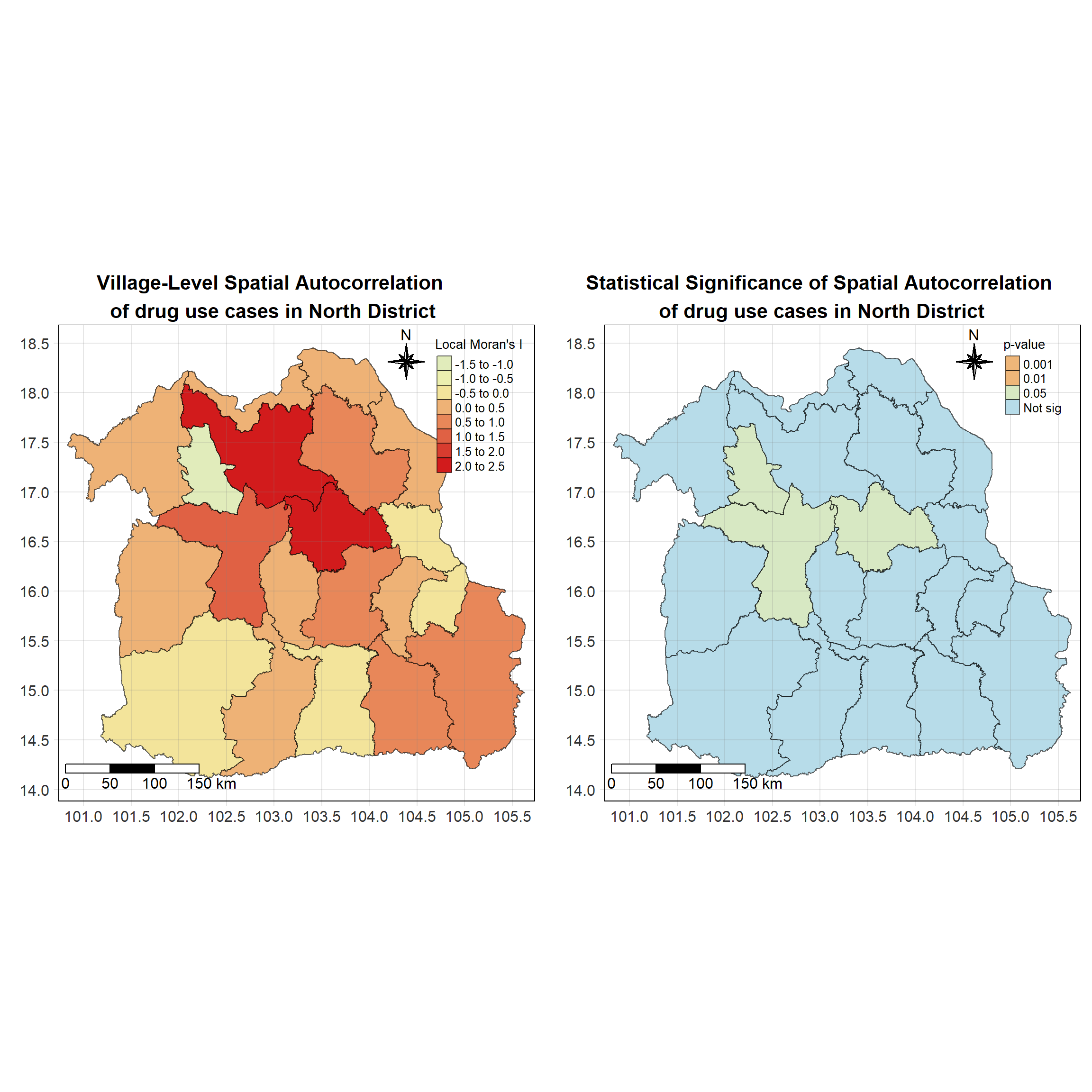

Northern Region

northern_local <- tm_shape(northern_lisa_2022)+
  tm_fill("ii", 
          palette = c("#e1ecbb","#f5f3a6", "#ec9a64","#de573e","#d21b1c"),
          title = "Local Moran's I",
          midpoint = NA) +
  tm_borders(col = "black", alpha = 0.6)+
  tm_layout(main.title = "Village-Level Spatial Autocorrelation \nof drug use cases in North District",
            main.title.position = "center",
            main.title.size = 1.3,
            main.title.fontface = "bold",
            legend.title.size = 1,
            legend.text.size = 0.8,
            frame = TRUE) +
  tm_borders(alpha = 0.5) +
  tm_compass(type="8star", text.size = 1, size = 2, position=c("RIGHT", "TOP")) +
  tm_scale_bar(position=c("LEFT", "BOTTOM"), text.size=1) +
  tm_grid(labels.size = 1,alpha =0.2)

northern_sig <- tm_shape(northern_lisa_2022)+
  tm_fill("p_ii_sim", 
          palette = c("#d21b1c","#ec9a64","#f5f3a6","#c9e3d2","#b7dce9"),
          breaks = c(0, 0.001, 0.01, 0.05, 1),
          labels = c("0.001", "0.01", "0.05", "Not sig"), 
          title = "p-value",
          midpoint = NA) +
  tm_borders(col = "black", alpha = 0.6)+
  tm_layout(main.title = "Statistical Significance of Spatial Autocorrelation\n of drug use cases in North District",
            main.title.position = "center",
            main.title.size = 1.3,
            main.title.fontface = "bold",
            legend.title.size = 1,
            legend.text.size = 0.8,
            frame = TRUE) +
  tm_borders(alpha = 0.5) +
  tm_compass(type="8star", text.size = 1, size = 2, position=c("RIGHT", "TOP")) +
  tm_scale_bar(position=c("LEFT", "BOTTOM"), text.size=1) +
  tm_grid(labels.size = 1,alpha =0.2)

tmap_arrange(northern_local,northern_sig, asp=1, ncol=2)

Western Region

western_local <- tm_shape(western_lisa_2022)+
  tm_fill("ii", 
          palette = c("#e1ecbb","#f5f3a6", "#ec9a64","#de573e","#d21b1c"),
          title = "Local Moran's I",
          midpoint = NA) +
  tm_borders(col = "black", alpha = 0.6)+
  tm_layout(main.title = "Village-Level Spatial Autocorrelation \nof drug use cases in North District",
            main.title.position = "center",
            main.title.size = 1.3,
            main.title.fontface = "bold",
            legend.title.size = 1,
            legend.text.size = 0.8,
            frame = TRUE) +
  tm_borders(alpha = 0.5) +
  tm_compass(type="8star", text.size = 1, size = 2, position=c("RIGHT", "TOP")) +
  tm_scale_bar(position=c("LEFT", "BOTTOM"), text.size=1) +
  tm_grid(labels.size = 1,alpha =0.2)

western_sig <- tm_shape(western_lisa_2022)+
  tm_fill("p_ii_sim", 
          palette = c("#d21b1c","#ec9a64","#f5f3a6","#c9e3d2","#b7dce9"),
          breaks = c(0, 0.001, 0.01, 0.05, 1),
          labels = c("0.001", "0.01", "0.05", "Not sig"), 
          title = "p-value",
          midpoint = NA) +
  tm_borders(col = "black", alpha = 0.6)+
  tm_layout(main.title = "Statistical Significance of Spatial Autocorrelation\n of drug use cases in North District",
            main.title.position = "center",
            main.title.size = 1.3,
            main.title.fontface = "bold",
            legend.title.size = 1,
            legend.text.size = 0.8,
            frame = TRUE) +
  tm_borders(alpha = 0.5) +
  tm_compass(type="8star", text.size = 1, size = 2, position=c("RIGHT", "TOP")) +
  tm_scale_bar(position=c("LEFT", "BOTTOM"), text.size=1) +
  tm_grid(labels.size = 1,alpha =0.2)

tmap_arrange(western_local,western_sig, asp=1, ncol=2)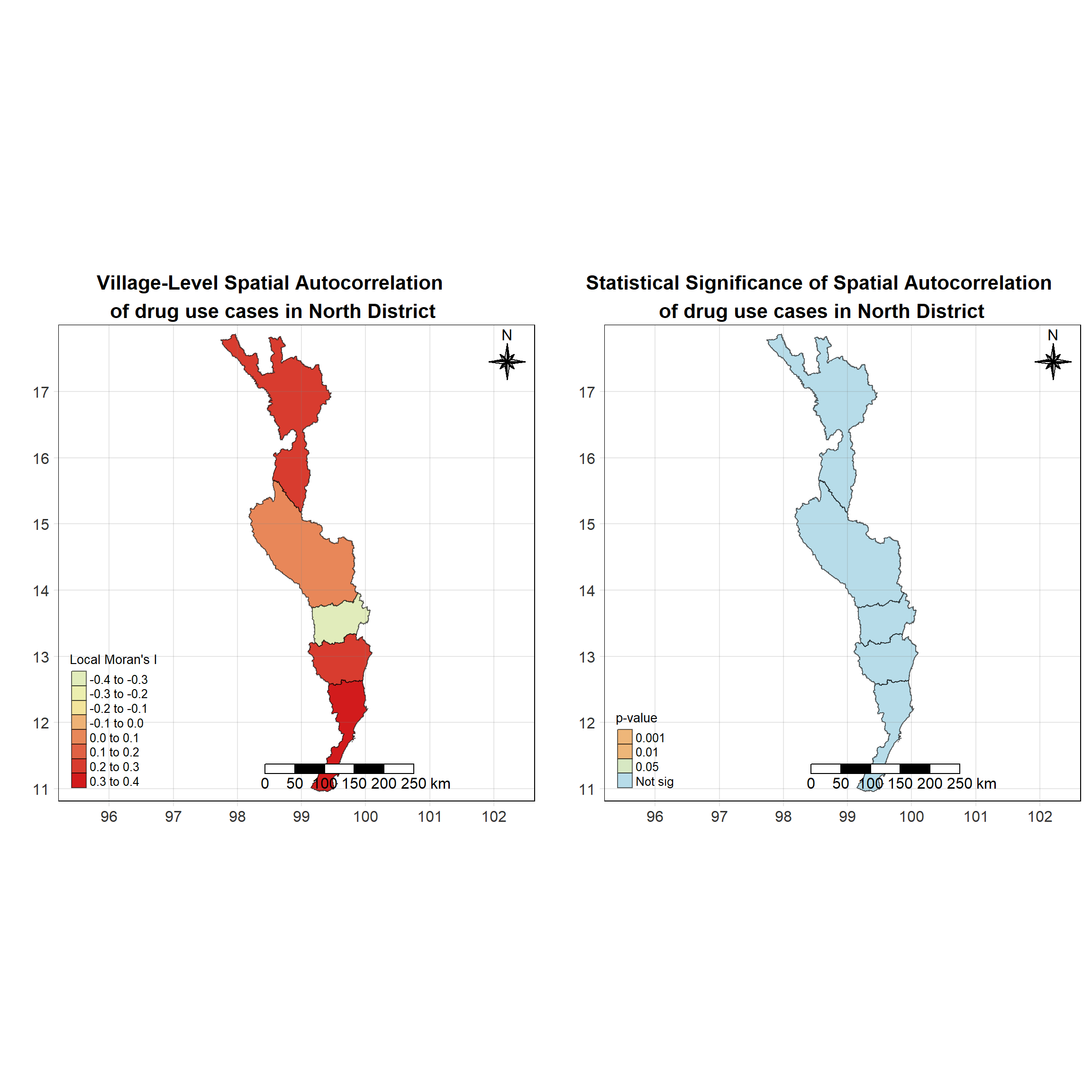

Central Region

central_local <- tm_shape(central_lisa_2022)+
  tm_fill("ii", 
          palette = c("#e1ecbb","#f5f3a6", "#ec9a64","#de573e","#d21b1c"),
          title = "Local Moran's I",
          midpoint = NA) +
  tm_borders(col = "black", alpha = 0.6)+
  tm_layout(main.title = "Village-Level Spatial Autocorrelation \nof drug use cases in North District",
            main.title.position = "center",
            main.title.size = 1.3,
            main.title.fontface = "bold",
            legend.title.size = 1,
            legend.text.size = 0.8,
            frame = TRUE) +
  tm_borders(alpha = 0.5) +
  tm_compass(type="8star", text.size = 1, size = 2, position=c("RIGHT", "TOP")) +
  tm_scale_bar(position=c("LEFT", "BOTTOM"), text.size=1) +
  tm_grid(labels.size = 1,alpha =0.2)

central_sig <- tm_shape(central_lisa_2022)+
  tm_fill("p_ii_sim", 
          palette = c("#d21b1c","#ec9a64","#f5f3a6","#c9e3d2","#b7dce9"),
          breaks = c(0, 0.001, 0.01, 0.05, 1),
          labels = c("0.001", "0.01", "0.05", "Not sig"), 
          title = "p-value",
          midpoint = NA) +
  tm_borders(col = "black", alpha = 0.6)+
  tm_layout(main.title = "Statistical Significance of Spatial Autocorrelation\n of drug use cases in North District",
            main.title.position = "center",
            main.title.size = 1.3,
            main.title.fontface = "bold",
            legend.title.size = 1,
            legend.text.size = 0.8,
            frame = TRUE) +
  tm_borders(alpha = 0.5) +
  tm_compass(type="8star", text.size = 1, size = 2, position=c("RIGHT", "TOP")) +
  tm_scale_bar(position=c("LEFT", "BOTTOM"), text.size=1) +
  tm_grid(labels.size = 1,alpha =0.2)

tmap_arrange(central_local,central_sig, asp=1, ncol=2)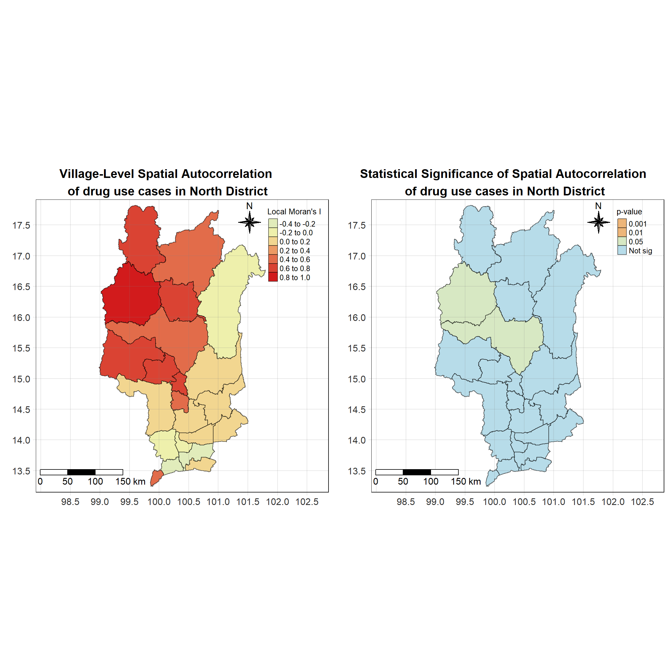

Eastern Region

eastern_local <- tm_shape(eastern_lisa_2022)+
  tm_fill("ii", 
          palette = c("#e1ecbb","#f5f3a6", "#ec9a64","#de573e","#d21b1c"),
          title = "Local Moran's I",
          midpoint = NA) +
  tm_borders(col = "black", alpha = 0.6)+
  tm_layout(main.title = "Village-Level Spatial Autocorrelation \nof drug use cases in North District",
            main.title.position = "center",
            main.title.size = 1.3,
            main.title.fontface = "bold",
            legend.title.size = 1,
            legend.text.size = 0.8,
            frame = TRUE) +
  tm_borders(alpha = 0.5) +
  tm_compass(type="8star", text.size = 1, size = 2, position=c("RIGHT", "TOP")) +
  tm_scale_bar(position=c("LEFT", "BOTTOM"), text.size=1) +
  tm_grid(labels.size = 1,alpha =0.2)

eastern_sig <- tm_shape(eastern_lisa_2022)+
  tm_fill("p_ii_sim", 
          palette = c("#d21b1c","#ec9a64","#f5f3a6","#c9e3d2","#b7dce9"),
          breaks = c(0, 0.001, 0.01, 0.05, 1),
          labels = c("0.001", "0.01", "0.05", "Not sig"), 
          title = "p-value",
          midpoint = NA) +
  tm_borders(col = "black", alpha = 0.6)+
  tm_layout(main.title = "Statistical Significance of Spatial Autocorrelation\n of drug use cases in North District",
            main.title.position = "center",
            main.title.size = 1.3,
            main.title.fontface = "bold",
            legend.title.size = 1,
            legend.text.size = 0.8,
            frame = TRUE) +
  tm_borders(alpha = 0.5) +
  tm_compass(type="8star", text.size = 1, size = 2, position=c("RIGHT", "TOP")) +
  tm_scale_bar(position=c("LEFT", "BOTTOM"), text.size=1) +
  tm_grid(labels.size = 1,alpha =0.2)

tmap_arrange(eastern_local,eastern_sig, asp=1, ncol=2)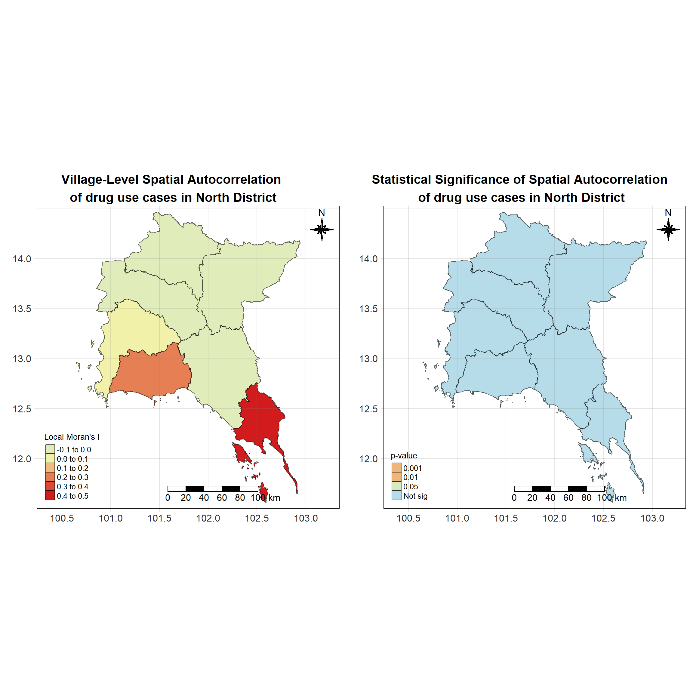

Southern Region

southern_local <- tm_shape(southern_lisa_2022)+
  tm_fill("ii", 
          palette = c("#e1ecbb","#f5f3a6", "#ec9a64","#de573e","#d21b1c"),
          title = "Local Moran's I",
          midpoint = NA) +
  tm_borders(col = "black", alpha = 0.6)+
  tm_layout(main.title = "Village-Level Spatial Autocorrelation \nof drug use cases in North District",
            main.title.position = "center",
            main.title.size = 1.3,
            main.title.fontface = "bold",
            legend.title.size = 1,
            legend.text.size = 0.8,
            frame = TRUE) +
  tm_borders(alpha = 0.5) +
  tm_compass(type="8star", text.size = 1, size = 2, position=c("RIGHT", "TOP")) +
  tm_scale_bar(position=c("LEFT", "BOTTOM"), text.size=1) +
  tm_grid(labels.size = 1,alpha =0.2)

southern_sig <- tm_shape(southern_lisa_2022)+
  tm_fill("p_ii_sim", 
          palette = c("#d21b1c","#ec9a64","#f5f3a6","#c9e3d2","#b7dce9"),
          breaks = c(0, 0.001, 0.01, 0.05, 1),
          labels = c("0.001", "0.01", "0.05", "Not sig"), 
          title = "p-value",
          midpoint = NA) +
  tm_borders(col = "black", alpha = 0.6)+
  tm_layout(main.title = "Statistical Significance of Spatial Autocorrelation\n of drug use cases in North District",
            main.title.position = "center",
            main.title.size = 1.3,
            main.title.fontface = "bold",
            legend.title.size = 1,
            legend.text.size = 0.8,
            frame = TRUE) +
  tm_borders(alpha = 0.5) +
  tm_compass(type="8star", text.size = 1, size = 2, position=c("RIGHT", "TOP")) +
  tm_scale_bar(position=c("LEFT", "BOTTOM"), text.size=1) +
  tm_grid(labels.size = 1,alpha =0.2)

tmap_arrange(southern_local,southern_sig, asp=1, ncol=2)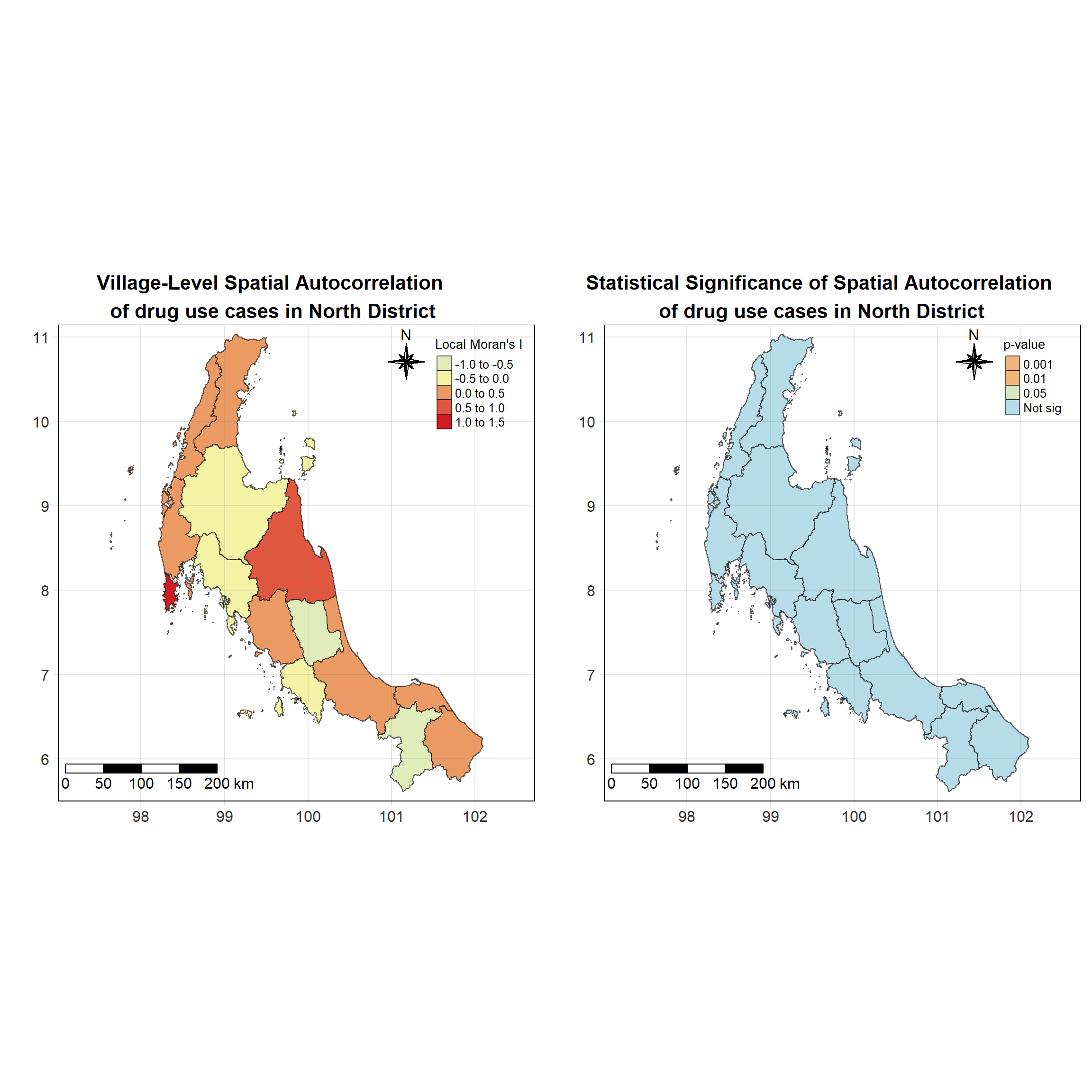

Analysis & Discussion

# Create the second map for northeastern_lisa_2022
northeastern_map <- tm_shape(northeastern_lisa_2022) +
  tm_polygons() +
  tm_borders(col = "black", alpha = 0.6) +
  tm_shape(northeastern_lisa_2022_sig) +
  tm_fill("mean", 
          palette = c("#b7dce9","#ec9a64","#e1ecbb", "#d21b1c"),
          title = "LISA class",
          midpoint = NA,
          legend.hist = TRUE, 
          legend.is.portrait = TRUE,
          legend.hist.z = 0.5) +
  tm_borders(col = "black", alpha = 0.6) +
  tm_layout(main.title = "2022 LISA plot of northeastern region",
            main.title.size = 0.8,
            legend.outside = TRUE)

# Create the first map for central_lisa_2022
central_map <- tm_shape(central_lisa_2022) +
  tm_polygons() +
  tm_borders(col = "black", alpha = 0.6) +
  tm_shape(central_lisa_2022_sig) +
  tm_fill("mean", 
          palette = c("#b7dce9","#ec9a64","#e1ecbb", "#d21b1c"),
          title = "LISA class",
          midpoint = NA,
          legend.hist = TRUE, 
          legend.is.portrait = TRUE,
          legend.hist.z = 0.5) +
  tm_borders(col = "black", alpha = 0.6) +
  tm_layout(main.title = "2022 LISA plot of central region",
            main.title.size = 0.8,
            legend.outside = TRUE)

# Arrange the two maps side by side
tmap_arrange(northeastern_map, central_map, asp=1, ncol=2)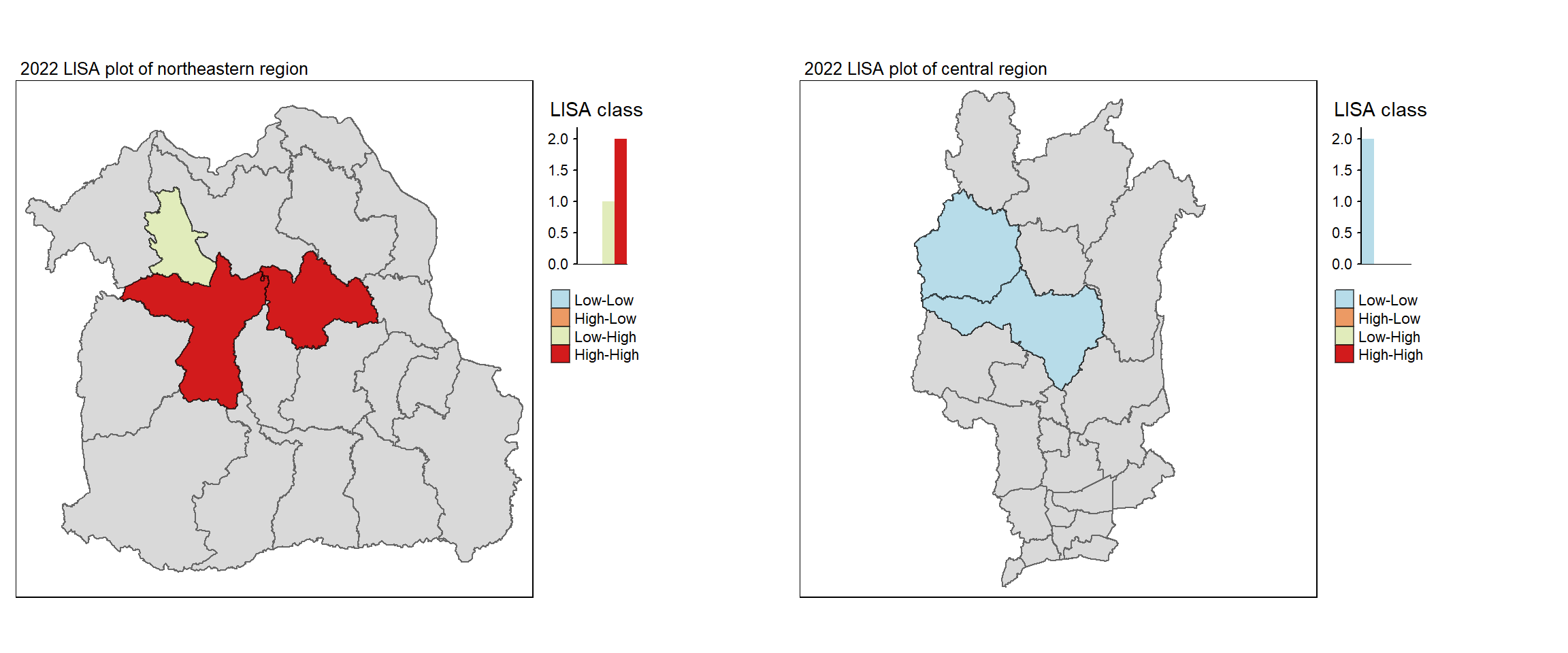

In 2022, the spatial autocorrelation patterns in the northeastern and central regions of Thailand present distinct shifts in drug use classifications compared to previous years.

In the Northeastern region (left plot), there is a notable concentration of High-High clusters, covering a few central provinces. This indicates that these provinces and their neighboring areas have higher-than-average drug-related cases, creating a significant hotspot. There is also a Low-High cluster in one province to the west of the hotspot. This pattern suggests that the province itself has low drug-related cases, but it is surrounded by high-value neighbors.

In the Central region (right plot), we observe a significant presence of Low-Low clusters in a few western and central provinces. Referencing the cluster data of 2021, this coldspot have consistently shown lower drug-related cases compared to the rest of the region.

Overall, the Northeastern region exhibits significant hotspots indicating provinces with elevated drug-related cases, which are surrounded by other high-case provinces. This is a marked contrast from the absence of such clusters in the Central region, which only shows Low-Low clusters representing coldspots.

The emergence of High-High clusters in the Northeastern region could point to new areas of concern that require targeted intervention strategies, while the presence of Low-Low clusters in the Central region suggests continued effectiveness in maintaining low levels of drug-related activities.

2.8 Hot Spot and Cold Spot Area Analysis

The Local Getis-Ord Gi* statistic is a spatial analysis technique used to identify hotspots and coldspots within geographic data. It measures spatial clustering by determining whether features with high or low values are spatially clustered.

2.8.1 Local Getis-Ord Gi for Hot Spot and Cold Spot Area Analysis

In the context of this analysis, Gi* helps identify areas with significantly high or low values of interest relative to their neighbors. A hotspot is an area where high values cluster, while a coldspot is where low values cluster.

Key aspects of the Getis-Ord Gi* statistic include:

1. Z-Scores and p-values: These indicate the statistical significance of the clustering. A high positive Gi* value with a low p-value suggests a hotspot, while a low negative Gi* value indicates a coldspot. Statistical significance is often represented using thresholds (e.g., p < 0.05).

2. Spatial Weighting: Gi* takes into account not just the value of the feature but also the values of neighboring features within a specified distance. The statistic compares the local mean to the global mean to assess whether clustering is due to chance or significant spatial patterns.

3. Application in Hotspot & Coldspot Analysis: In this analysis, the Gi* statistic is applied to geographical areas to identify statistically significant areas of unusually high or low values of the phenomenon under study, such as drug use cases. These areas can then be visualized using a color scale, helping researchers or decision-makers focus on regions that exhibit non-random spatial patterns.

By visualizing Gi* results on a map, we can better understand the spatial dynamics of an issue and prioritize interventions in areas of concern.

We start by calculating Inverse Distance Weighted (IDW) spatial weight matrices for the years 2017-2022 using contiguity-based neighborhoods. Each region is considered as its own neighbor (with include_self), and spatial weights are assigned based on the inverse distance between regions (st_inverse_distance), giving more weight to closer regions. This creates a foundation for spatial autocorrelation analysis by providing the necessary spatial relationships for each year.

wm_idw_2017 <- region_2017_sf %>%
  mutate(nb = include_self(st_contiguity(geometry)),
         wt = st_inverse_distance(nb, geometry,
                                   scale = 1,
                                   alpha = 1),
         .before = 1)
wm_idw_2018 <- region_2018_sf %>%
  mutate(nb = include_self(st_contiguity(geometry)),
         wt = st_inverse_distance(nb, geometry,
                                   scale = 1,
                                   alpha = 1),
         .before = 1)
wm_idw_2019 <- region_2019_sf %>%
  mutate(nb = include_self(st_contiguity(geometry)),
         wt = st_inverse_distance(nb, geometry,
                                   scale = 1,
                                   alpha = 1),
         .before = 1)
wm_idw_2020 <- region_2020_sf %>%
  mutate(nb = include_self(st_contiguity(geometry)),
         wt = st_inverse_distance(nb, geometry,
                                   scale = 1,
                                   alpha = 1),
         .before = 1)
wm_idw_2021 <- region_2021_sf %>%
  mutate(nb = include_self(st_contiguity(geometry)),
         wt = st_inverse_distance(nb, geometry,
                                   scale = 1,
                                   alpha = 1),
         .before = 1)
wm_idw_2022 <- region_2022_sf %>%
  mutate(nb = include_self(st_contiguity(geometry)),
         wt = st_inverse_distance(nb, geometry,
                                   scale = 1,
                                   alpha = 1),
         .before = 1)

We store the yearly spatial weight matrices for ease of use

write_rds(wm_idw_2017, "data/rds/wm_idw_2017.rds")
write_rds(wm_idw_2018, "data/rds/wm_idw_2018.rds")
write_rds(wm_idw_2019, "data/rds/wm_idw_2019.rds")
write_rds(wm_idw_2020, "data/rds/wm_idw_2020.rds")
write_rds(wm_idw_2021, "data/rds/wm_idw_2021.rds")
write_rds(wm_idw_2022, "data/rds/wm_idw_2022.rds")

wm_idw_2017 <- read_rds("data/rds/wm_idw_2017.rds")
wm_idw_2018 <- read_rds("data/rds/wm_idw_2018.rds")
wm_idw_2019 <- read_rds("data/rds/wm_idw_2019.rds")
wm_idw_2020 <- read_rds("data/rds/wm_idw_2020.rds")
wm_idw_2021 <- read_rds("data/rds/wm_idw_2021.rds")
wm_idw_2022 <- read_rds("data/rds/wm_idw_2022.rds")

We apply the Local Getis-Ord Gi* statistic to identify spatial clusters (hotspots and coldspots) of cases for each year (2017-2022) onto the yearly spatial weight matrices. Using the local_gstar_perm() function, it calculates Gi values for each region, based on the case counts (no_cases), spatial neighbors (nb), and their corresponding weights (wt), with 99 Monte Carlo simulations (nsim = 99) for statistical significance. The results are then added back to the dataset for visualization and further analysis.

set.seed(4242)

HCSA_2017 <- wm_idw_2017 %>% 
  mutate(local_Gi_star = local_gstar_perm(
    no_cases, nb, wt, nsim = 99),
         .before = 1) %>%
  unnest(local_Gi_star)
HCSA_2018 <- wm_idw_2018 %>% 
  mutate(local_Gi_star = local_gstar_perm(
    no_cases, nb, wt, nsim = 99),
         .before = 1) %>%
  unnest(local_Gi_star)
HCSA_2018 <- wm_idw_2018 %>% 
  mutate(local_Gi_star = local_gstar_perm(
    no_cases, nb, wt, nsim = 99),
         .before = 1) %>%
  unnest(local_Gi_star)
HCSA_2019 <- wm_idw_2019 %>% 
  mutate(local_Gi_star = local_gstar_perm(
    no_cases, nb, wt, nsim = 99),
         .before = 1) %>%
  unnest(local_Gi_star)
HCSA_2020 <- wm_idw_2020 %>% 
  mutate(local_Gi_star = local_gstar_perm(
    no_cases, nb, wt, nsim = 99),
         .before = 1) %>%
  unnest(local_Gi_star)
HCSA_2021 <- wm_idw_2021 %>% 
  mutate(local_Gi_star = local_gstar_perm(
    no_cases, nb, wt, nsim = 99),
         .before = 1) %>%
  unnest(local_Gi_star)
HCSA_2022 <- wm_idw_2022 %>% 
  mutate(local_Gi_star = local_gstar_perm(
    no_cases, nb, wt, nsim = 99),
         .before = 1) %>%
  unnest(local_Gi_star)

2017

Map of Hotspots & Coldspots of Drug Use Cases in Thailand

First we generate a map of Thailand for the current year, showing the hotspots and coldspots of drug use cases using Gi statistics. The fill color is determined by the gi_star column using a specified color palette, with a midpoint of 0 to distinguish between hotspots (positive Gi) and coldspots (negative Gi). The map also includes borders, a title, a compass, a scale bar, and a grid.

tm_shape(HCSA_2017)+
  tm_fill("gi_star", 
          palette = c("#57bfc0", "#7977f3","#f8d673","#f8b675","#f67774"),
          title = "Gi*",
          midpoint = 0) +
  tm_borders(col = "black", alpha = 0.6)+
  tm_layout(main.title = "2017 Hotspots & Coldspots of drug\n use cases in Thailand",
            main.title.position = "center",
            main.title.size = 1.7,
            main.title.fontface = "bold",
            legend.title.size = 1.8,
            legend.text.size = 1.3,
            legend.outside = TRUE,
            frame = TRUE) +
  tm_borders(alpha = 0.5) +
  tm_compass(type="8star", text.size = 1.5, size = 3, position=c("RIGHT", "TOP")) +
  tm_scale_bar(position=c("LEFT", "BOTTOM"), text.size=1.2) +
  tm_grid(labels.size = 1,alpha =0.2)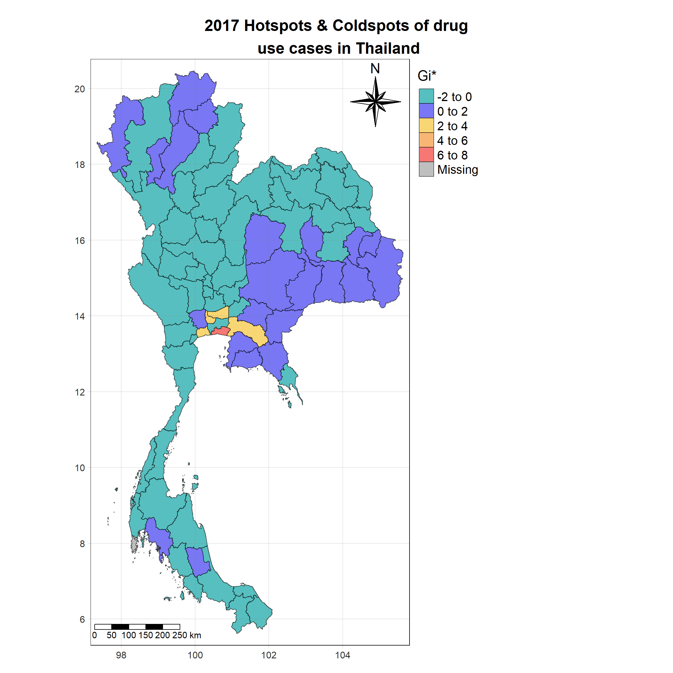

Map of Statistically Significant Hotspots & Coldspots of Drug Use Cases

We then create a map similar to the previous one but filters the data to only show provinces where the p_sim value is less than 0.05 (indicating statistically significant results). It visualizes the statistically significant hotspots and coldspots, with gi_star values categorized into specific intervals (breaks = c(-2, 0, 2, 4, 6, 8)), and includes a histogram in the legend for distribution reference.

HCSA_2017_sig <- HCSA_2017  %>%
  filter(p_sim < 0.05)

tm_shape(HCSA_2017) +
  tm_polygons() +
tm_shape(HCSA_2017_sig)+
  tm_fill("gi_star", 
          title = "Gi*",
          palette = c("#57bfc0", "#7977f3","#f8d673","#f8b675","#f67774"),
          breaks = c(-2, 0, 2, 4, 6, 8), 
          midpoint = 0,
          legend.hist = TRUE, 
          legend.is.portrait = TRUE,
          legend.hist.z = 0.1) +
  tm_borders(col = "black", alpha = 0.6)+
  tm_layout(main.title = "Statistically Significant Hotspots & Coldspots \nof Drug use cases in Thailand",
            main.title.position = "center",
            main.title.size = 1.7,
            main.title.fontface = "bold",
            legend.title.size = 1.8,
            legend.text.size = 1.3,
            legend.outside = TRUE,
            frame = TRUE) +
  tm_borders(alpha = 0.5) +
  tm_compass(type="8star", text.size = 1.5, size = 3, position=c("RIGHT", "TOP")) +
  tm_scale_bar(position=c("LEFT", "BOTTOM"), text.size=1.2) +
  tm_grid(labels.size = 1,alpha =0.2)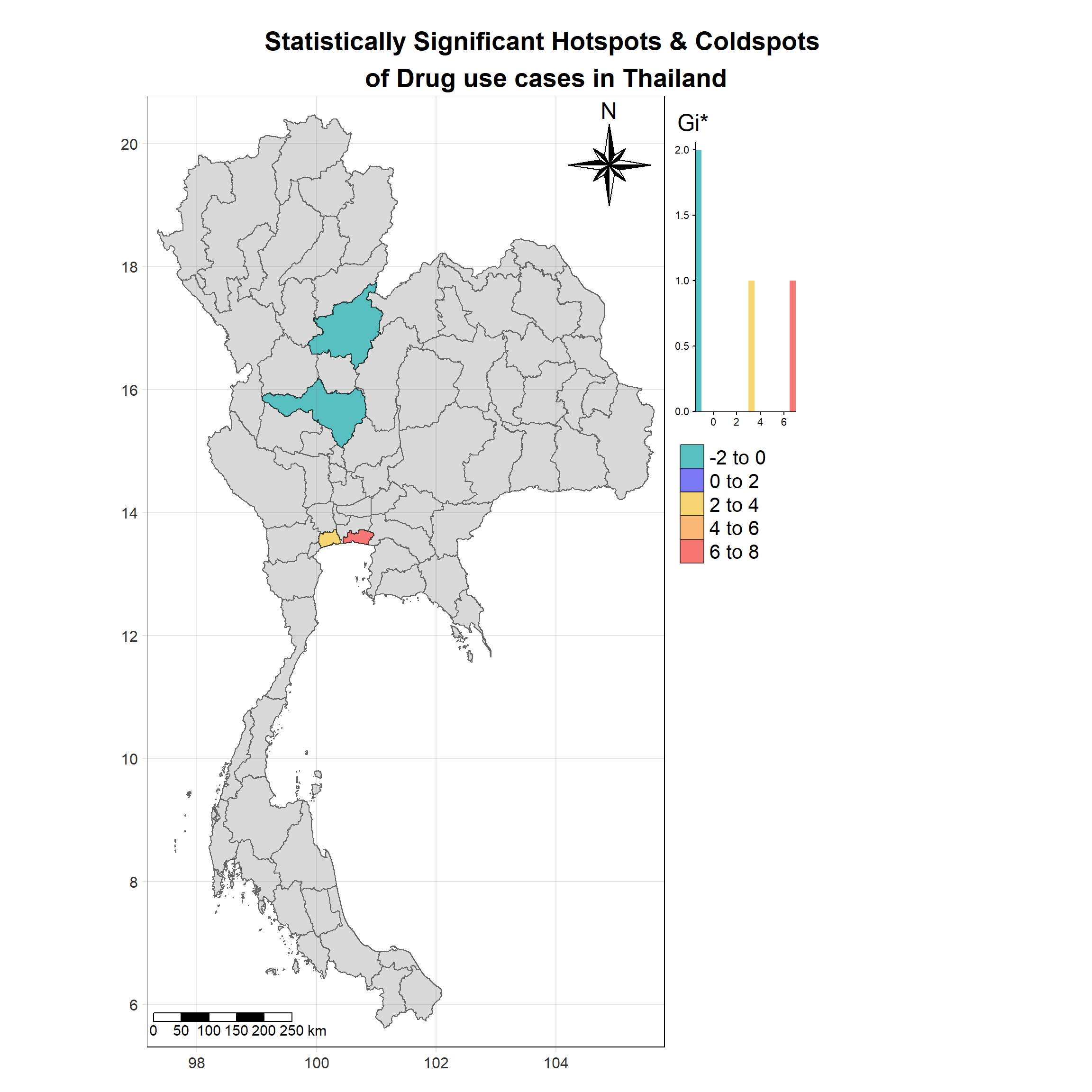

Top Hotspots and Coldspots Identification

We then identify the top hotspot provinces (with the highest positive gi_star values) and the top coldspot provinces (with the lowest negative gi_star values). It uses the filtered HCSA_<current_year>_sig dataset and arranges the values in descending and ascending order, respectively, to extract the top provinces.

# Get the top 3 hotspots (highest positive gi_star values)
top_hotspots <- HCSA_2017_sig %>%
  arrange(desc(gi_star)) %>%
  head(3) %>%
  pull(province_en)

# Get the top 3 cold spots (lowest negative gi_star values)
top_coldspots <- HCSA_2017_sig %>%
  filter(!(province_en %in% top_hotspots)) %>%
  arrange(gi_star) %>%
  head(3) %>%
  pull(province_en)

HCSA_top_hotspots <- HCSA_2017_sig %>% filter(province_en %in% top_hotspots)
HCSA_top_coldspots <- HCSA_2017_sig %>% filter(province_en %in% top_coldspots)

tm_shape(HCSA_2017) +
  tm_polygons() +
tm_shape(HCSA_top_hotspots)+
  tm_fill("gi_star", 
          palette = c("#f67774")) +
  tm_borders(col = "black", alpha = 0.6)+
  tm_text("province_en",auto.placement = T)+
  tm_layout(main.title = "Most Significant Hotspots of Drug use\n cases in Thailand",
            main.title.position = "center",
            main.title.size = 1.7,
            main.title.fontface = "bold",
            legend.show = FALSE,
            frame = TRUE) +
  tm_borders(alpha = 0.5) +
  tm_compass(type="8star", text.size = 1.5, size = 3, position=c("RIGHT", "TOP")) +
  tm_scale_bar(position=c("LEFT", "BOTTOM"), text.size=1.2) +
  tm_grid(labels.size = 1,alpha =0.2)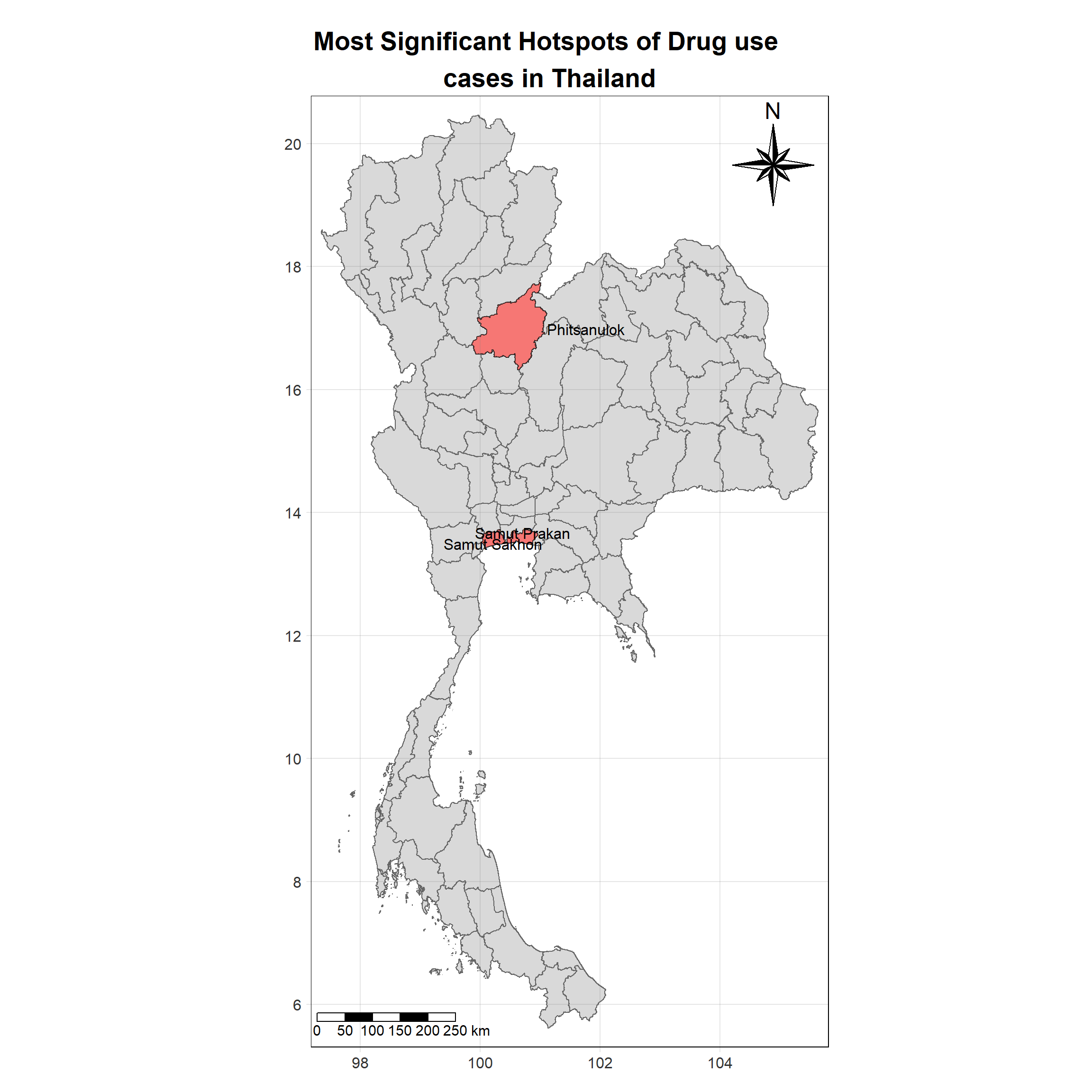

tm_shape(HCSA_2017) +
  tm_polygons() +
tm_shape(HCSA_top_coldspots)+
  tm_fill("gi_star", 
          palette = c("#57bfc0")) +
  tm_borders(col = "black", alpha = 0.6)+
  tm_text("province_en", auto.placement = T)+
  tm_layout(main.title = "Most Significant Coldspots of Drug use\n cases in Thailand",
            main.title.position = "center",
            main.title.size = 1.7,
            main.title.fontface = "bold",
            legend.show = FALSE,
            frame = TRUE) +
  tm_borders(alpha = 0.5) +
  tm_compass(type="8star", text.size = 1.5, size = 3, position=c("RIGHT", "TOP")) +
  tm_scale_bar(position=c("LEFT", "BOTTOM"), text.size=1.2) +
  tm_grid(labels.size = 1,alpha =0.2)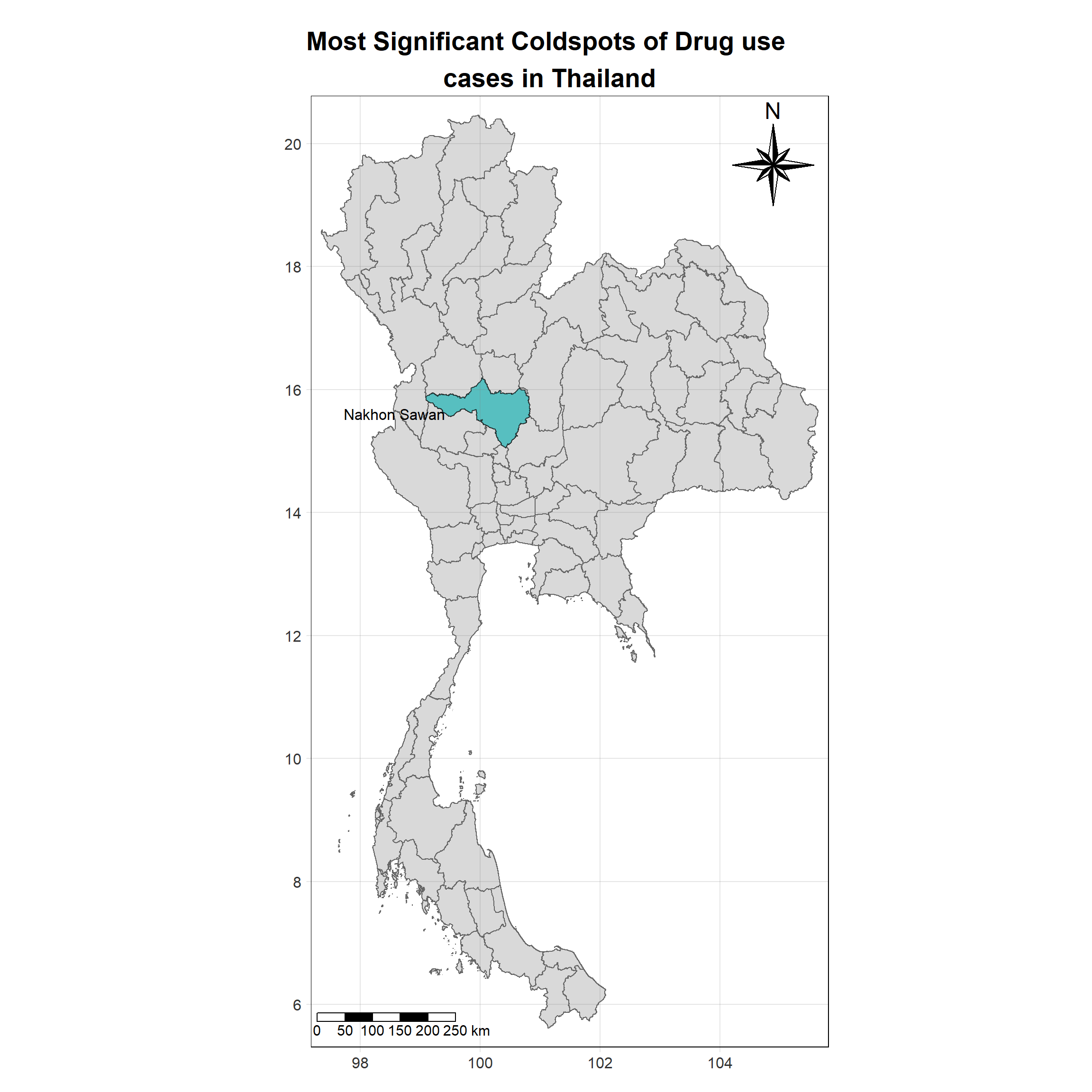

2018

Map of Hotspots & Coldspots of Drug Use Cases in Thailand

First we generate a map of Thailand for the current year, showing the hotspots and coldspots of drug use cases using Gi statistics. The fill color is determined by the gi_star column using a specified color palette, with a midpoint of 0 to distinguish between hotspots (positive Gi) and coldspots (negative Gi). The map also includes borders, a title, a compass, a scale bar, and a grid.

tm_shape(HCSA_2018)+
  tm_fill("gi_star", 
          palette = c("#57bfc0", "#7977f3","#f8d673","#f8b675","#f67774"),
          title = "Gi*",
          midpoint = 0) +
  tm_borders(col = "black", alpha = 0.6)+
  tm_layout(main.title = "2018 Hotspots & Coldspots of drug\n use cases in Thailand",
            main.title.position = "center",
            main.title.size = 1.7,
            main.title.fontface = "bold",
            legend.title.size = 1.8,
            legend.text.size = 1.3,
            legend.outside = TRUE,
            frame = TRUE) +
  tm_borders(alpha = 0.5) +
  tm_compass(type="8star", text.size = 1.5, size = 3, position=c("RIGHT", "TOP")) +
  tm_scale_bar(position=c("LEFT", "BOTTOM"), text.size=1.2) +
  tm_grid(labels.size = 1,alpha =0.2)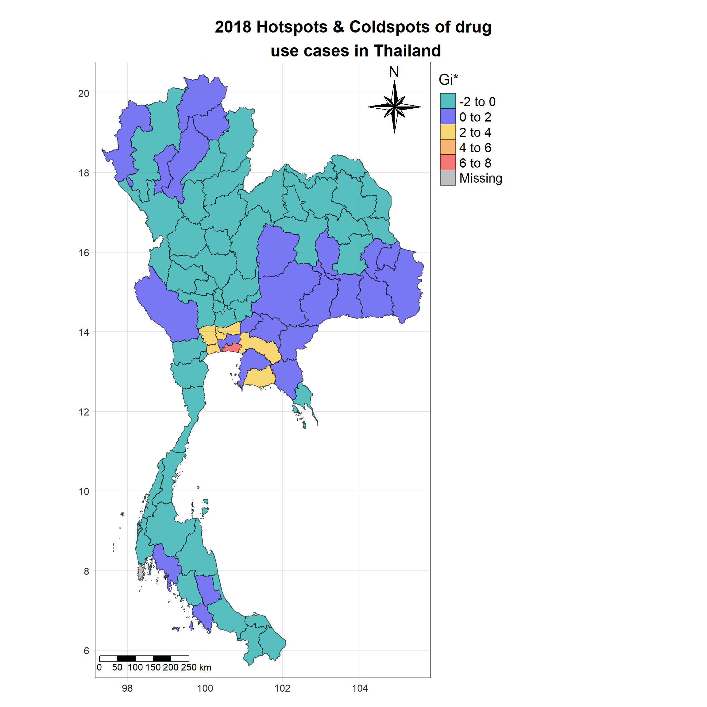

Map of Statistically Significant Hotspots & Coldspots of Drug Use Cases

We then create a map similar to the previous one but filters the data to only show provinces where the p_sim value is less than 0.05 (indicating statistically significant results). It visualizes the statistically significant hotspots and coldspots, with gi_star values categorized into specific intervals (breaks = c(-2, 0, 2, 4, 6, 8)), and includes a histogram in the legend for distribution reference.

HCSA_2018_sig <- HCSA_2018  %>%
  filter(p_sim < 0.05)

tm_shape(HCSA_2018) +
  tm_polygons() +
tm_shape(HCSA_2018_sig)+
  tm_fill("gi_star", 
          title = "Gi*",
          palette = c("#57bfc0", "#7977f3","#f8d673","#f8b675","#f67774"),
          breaks = c(-2, 0, 2, 4, 6, 8), 
          midpoint = 0,
          legend.hist = TRUE, 
          legend.is.portrait = TRUE,
          legend.hist.z = 0.1) +
  tm_borders(col = "black", alpha = 0.6)+
  tm_layout(main.title = "Statistically Significant Hotspots & Coldspots \nof Drug use cases in Thailand",
            main.title.position = "center",
            main.title.size = 1.7,
            main.title.fontface = "bold",
            legend.title.size = 1.8,
            legend.text.size = 1.3,
            legend.outside = TRUE,
            frame = TRUE) +
  tm_borders(alpha = 0.5) +
  tm_compass(type="8star", text.size = 1.5, size = 3, position=c("RIGHT", "TOP")) +
  tm_scale_bar(position=c("LEFT", "BOTTOM"), text.size=1.2) +
  tm_grid(labels.size = 1,alpha =0.2)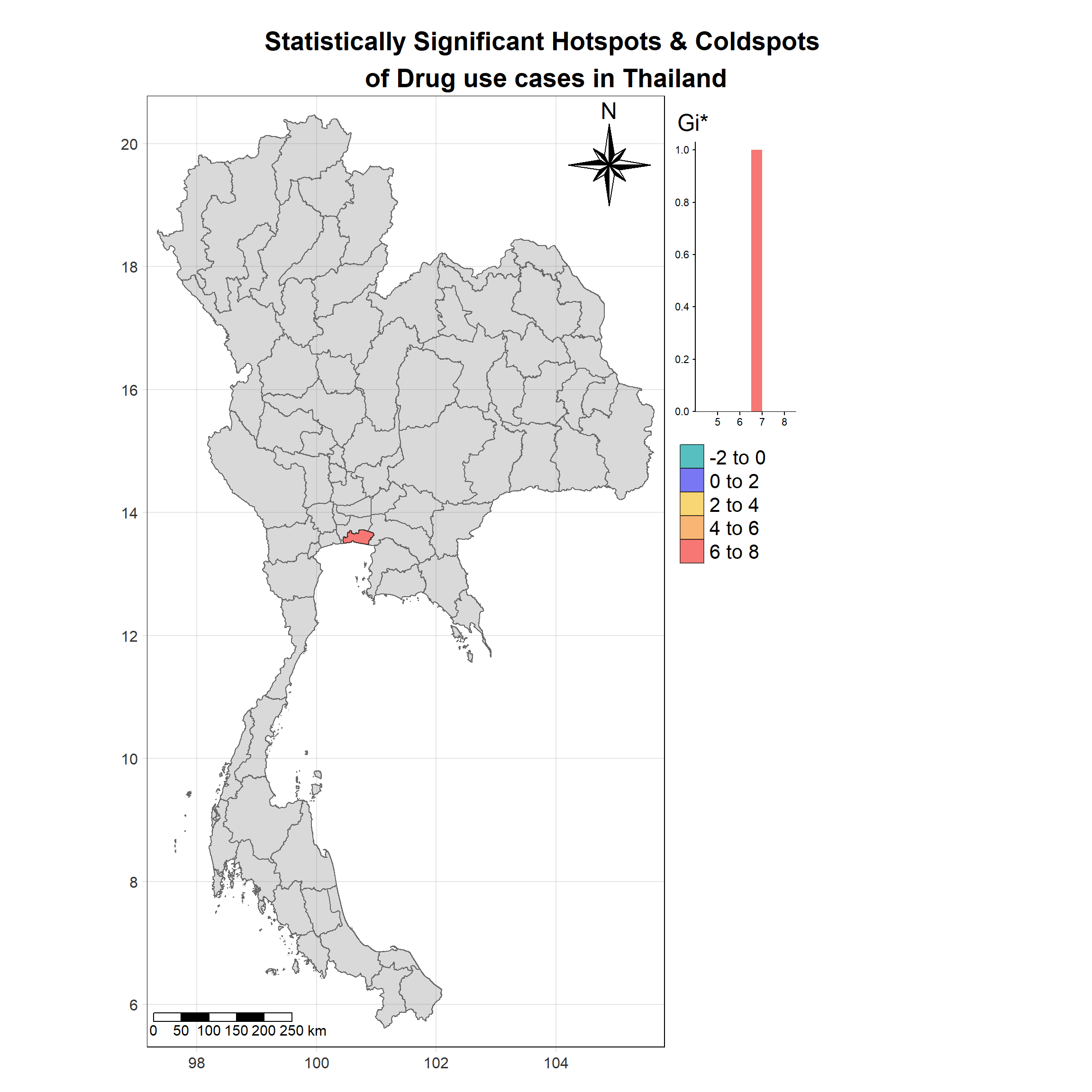

Top Hotspots and Coldspots Identification

We then identify the top hotspot provinces (with the highest positive gi_star values) and the top coldspot provinces (with the lowest negative gi_star values). It uses the filtered HCSA_<current_year>_sig dataset and arranges the values in descending and ascending order, respectively, to extract the top provinces.

From the plot above, it, there is only 1 statistically significant hotspot during the year 2018. We will get the top hotspot based on gi_star value.

# Get the top hotspot (highest positive gi_star values)
top_hotspots <- HCSA_2018_sig %>%
  arrange(desc(gi_star)) %>%
  head(1) %>%
  pull(province_en)

HCSA_top_hotspots <- HCSA_2018_sig %>% filter(province_en %in% top_hotspots)
HCSA_top_coldspots <- HCSA_2018_sig %>% filter(province_en %in% top_coldspots)

tm_shape(HCSA_2018) +
  tm_polygons() +
tm_shape(HCSA_top_hotspots)+
  tm_fill("gi_star", 
          palette = c("#f67774")) +
  tm_borders(col = "black", alpha = 0.6)+
  tm_text("province_en",auto.placement = T)+
  tm_layout(main.title = "Most Significant Hotspots of Drug use\n cases in Thailand",
            main.title.position = "center",
            main.title.size = 1.7,
            main.title.fontface = "bold",
            legend.show = FALSE,
            frame = TRUE) +
  tm_borders(alpha = 0.5) +
  tm_compass(type="8star", text.size = 1.5, size = 3, position=c("RIGHT", "TOP")) +
  tm_scale_bar(position=c("LEFT", "BOTTOM"), text.size=1.2) +
  tm_grid(labels.size = 1,alpha =0.2)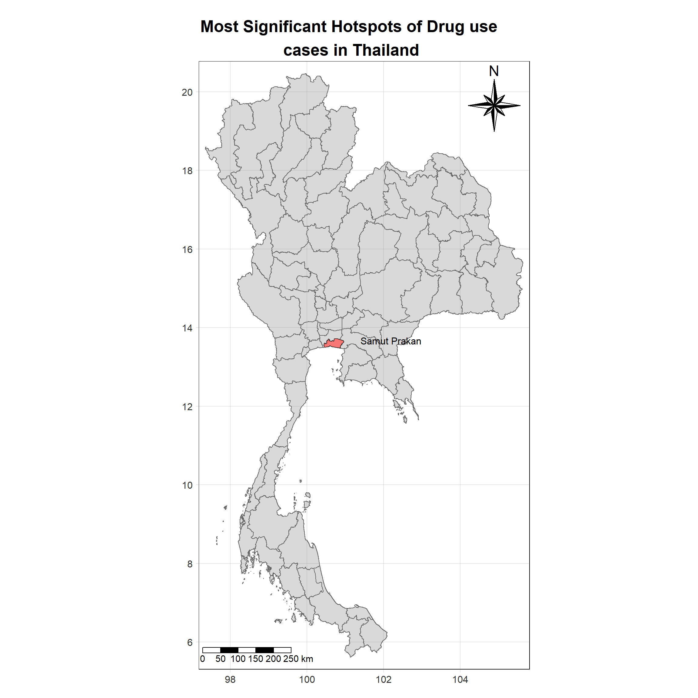

2019

Map of Hotspots & Coldspots of Drug Use Cases in Thailand

First we generate a map of Thailand for the current year, showing the hotspots and coldspots of drug use cases using Gi statistics. The fill color is determined by the gi_star column using a specified color palette, with a midpoint of 0 to distinguish between hotspots (positive Gi) and coldspots (negative Gi). The map also includes borders, a title, a compass, a scale bar, and a grid.

tm_shape(HCSA_2019)+
  tm_fill("gi_star", 
          palette = c("#57bfc0", "#7977f3","#f8d673","#f8b675","#f67774"),
          title = "Gi*",
          midpoint = 0) +
  tm_borders(col = "black", alpha = 0.6)+
  tm_layout(main.title = "2019 Hotspots & Coldspots of drug\n use cases in Thailand",
            main.title.position = "center",
            main.title.size = 1.7,
            main.title.fontface = "bold",
            legend.title.size = 1.8,
            legend.text.size = 1.3,
            legend.outside = TRUE,
            frame = TRUE) +
  tm_borders(alpha = 0.5) +
  tm_compass(type="8star", text.size = 1.5, size = 3, position=c("RIGHT", "TOP")) +
  tm_scale_bar(position=c("LEFT", "BOTTOM"), text.size=1.2) +
  tm_grid(labels.size = 1,alpha =0.2)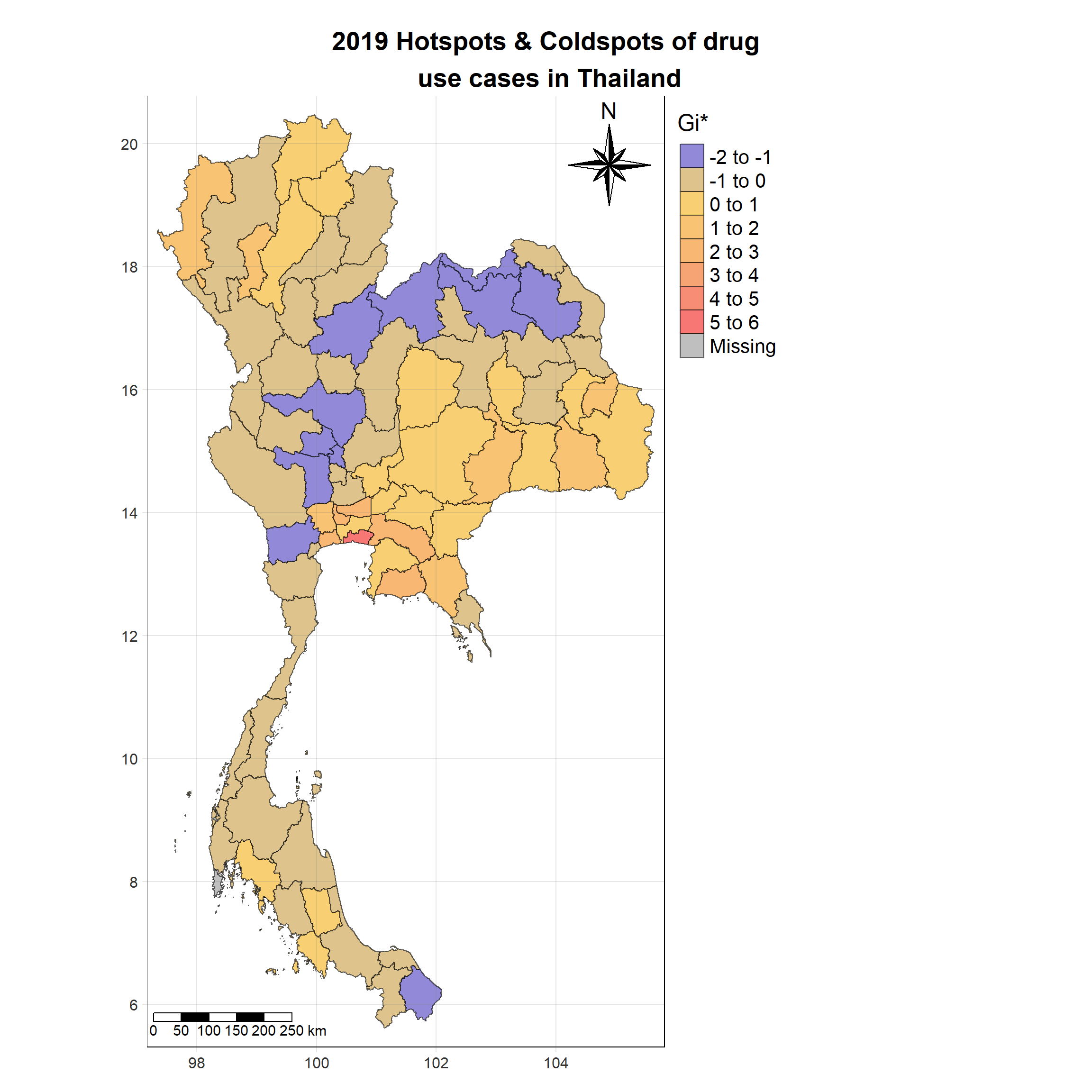

Map of Statistically Significant Hotspots & Coldspots of Drug Use Cases

We then create a map similar to the previous one but filters the data to only show provinces where the p_sim value is less than 0.05 (indicating statistically significant results). It visualizes the statistically significant hotspots and coldspots, with gi_star values categorized into specific intervals (breaks = c(-2, 0, 2, 4, 6, 8)), and includes a histogram in the legend for distribution reference.

HCSA_2019_sig <- HCSA_2019  %>%
  filter(p_sim < 0.05)

tm_shape(HCSA_2019) +
  tm_polygons() +
tm_shape(HCSA_2019_sig)+
  tm_fill("gi_star", 
          title = "Gi*",
          palette = c("#57bfc0", "#7977f3","#f8d673","#f8b675","#f67774"),
          breaks = c(-2, 0, 2, 4, 6, 8), 
          midpoint = 0,
          legend.hist = TRUE, 
          legend.is.portrait = TRUE,
          legend.hist.z = 0.1) +
  tm_borders(col = "black", alpha = 0.6)+
  tm_layout(main.title = "Statistically Significant Hotspots & Coldspots \nof Drug use cases in Thailand",
            main.title.position = "center",
            main.title.size = 1.7,
            main.title.fontface = "bold",
            legend.title.size = 1.8,
            legend.text.size = 1.3,
            legend.outside = TRUE,
            frame = TRUE) +
  tm_borders(alpha = 0.5) +
  tm_compass(type="8star", text.size = 1.5, size = 3, position=c("RIGHT", "TOP")) +
  tm_scale_bar(position=c("LEFT", "BOTTOM"), text.size=1.2) +
  tm_grid(labels.size = 1,alpha =0.2)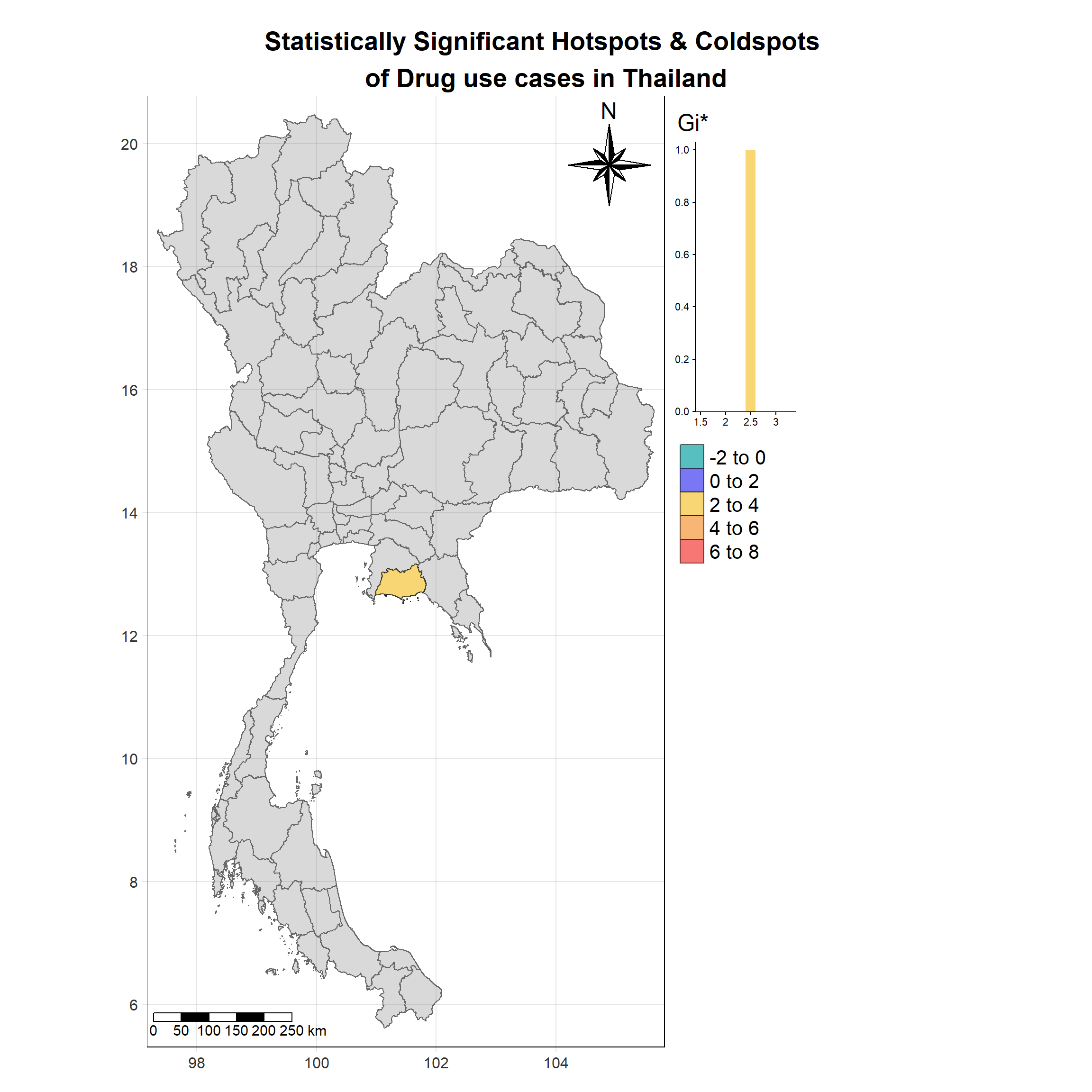

Top Hotspots and Coldspots Identification

We then identify the top hotspot provinces (with the highest positive gi_star values) and the top coldspot provinces (with the lowest negative gi_star values). It uses the filtered HCSA_<current_year>_sig dataset and arranges the values in descending and ascending order, respectively, to extract the top provinces.

From the plot above, it, there is only 1 statistically significant hotspot during the year 2018. We will get the top hotspot based on gi_star value.

# Get the top hotspot (highest positive gi_star values)
top_hotspots <- HCSA_2019_sig %>%
  arrange(desc(gi_star)) %>%
  head(1) %>%
  pull(province_en)

HCSA_top_hotspots <- HCSA_2019_sig %>% filter(province_en %in% top_hotspots)
HCSA_top_coldspots <- HCSA_2019_sig %>% filter(province_en %in% top_coldspots)

tm_shape(HCSA_2019) +
  tm_polygons() +
tm_shape(HCSA_top_hotspots)+
  tm_fill("gi_star", 
          palette = c("#f67774")) +
  tm_borders(col = "black", alpha = 0.6)+
  tm_text("province_en",auto.placement = T)+
  tm_layout(main.title = "Most Significant Hotspots of Drug use\n cases in Thailand",
            main.title.position = "center",
            main.title.size = 1.7,
            main.title.fontface = "bold",
            legend.show = FALSE,
            frame = TRUE) +
  tm_borders(alpha = 0.5) +
  tm_compass(type="8star", text.size = 1.5, size = 3, position=c("RIGHT", "TOP")) +
  tm_scale_bar(position=c("LEFT", "BOTTOM"), text.size=1.2) +
  tm_grid(labels.size = 1,alpha =0.2)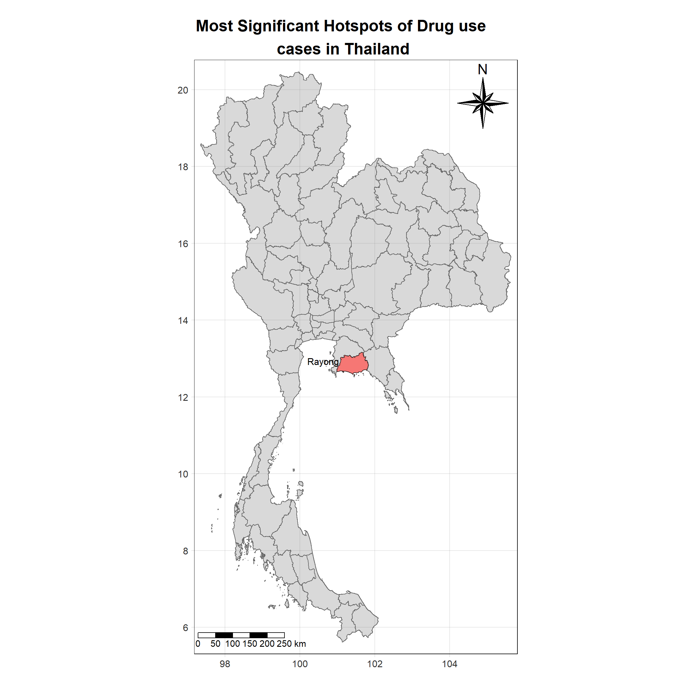

2020

Map of Hotspots & Coldspots of Drug Use Cases in Thailand

First we generate a map of Thailand for the current year, showing the hotspots and coldspots of drug use cases using Gi statistics. The fill color is determined by the gi_star column using a specified color palette, with a midpoint of 0 to distinguish between hotspots (positive Gi) and coldspots (negative Gi). The map also includes borders, a title, a compass, a scale bar, and a grid.

tm_shape(HCSA_2020)+
  tm_fill("gi_star", 
          palette = c("#57bfc0", "#7977f3","#f8d673","#f8b675","#f67774"),
          title = "Gi*",
          midpoint = 0) +
  tm_borders(col = "black", alpha = 0.6)+
  tm_layout(main.title = "2020 Hotspots & Coldspots of drug\n use cases in Thailand",
            main.title.position = "center",
            main.title.size = 1.7,
            main.title.fontface = "bold",
            legend.title.size = 1.8,
            legend.text.size = 1.3,
            legend.outside = TRUE,
            frame = TRUE) +
  tm_borders(alpha = 0.5) +
  tm_compass(type="8star", text.size = 1.5, size = 3, position=c("RIGHT", "TOP")) +
  tm_scale_bar(position=c("LEFT", "BOTTOM"), text.size=1.2) +
  tm_grid(labels.size = 1,alpha =0.2)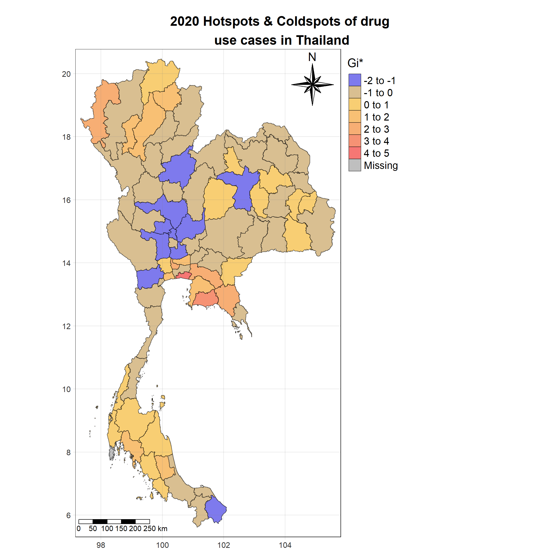

Map of Statistically Significant Hotspots & Coldspots of Drug Use Cases

We then create a map similar to the previous one but filters the data to only show provinces where the p_sim value is less than 0.05 (indicating statistically significant results). It visualizes the statistically significant hotspots and coldspots, with gi_star values categorized into specific intervals (breaks = c(-2, 0, 2, 4, 6, 8)), and includes a histogram in the legend for distribution reference.

HCSA_2020_sig <- HCSA_2020  %>%
  filter(p_sim < 0.05)

tm_shape(HCSA_2020) +
  tm_polygons() +
tm_shape(HCSA_2020_sig)+
  tm_fill("gi_star", 
          title = "Gi*",
          palette = c("#57bfc0", "#7977f3","#f8d673","#f8b675","#f67774"),
          breaks = c(-2, 0, 2, 4, 6, 8), 
          midpoint = 0,
          legend.hist = TRUE, 
          legend.is.portrait = TRUE,
          legend.hist.z = 0.1) +
  tm_borders(col = "black", alpha = 0.6)+
  tm_layout(main.title = "Statistically Significant Hotspots & Coldspots \nof Drug use cases in Thailand",
            main.title.position = "center",
            main.title.size = 1.7,
            main.title.fontface = "bold",
            legend.title.size = 1.8,
            legend.text.size = 1.3,
            legend.outside = TRUE,
            frame = TRUE) +
  tm_borders(alpha = 0.5) +
  tm_compass(type="8star", text.size = 1.5, size = 3, position=c("RIGHT", "TOP")) +
  tm_scale_bar(position=c("LEFT", "BOTTOM"), text.size=1.2) +
  tm_grid(labels.size = 1,alpha =0.2)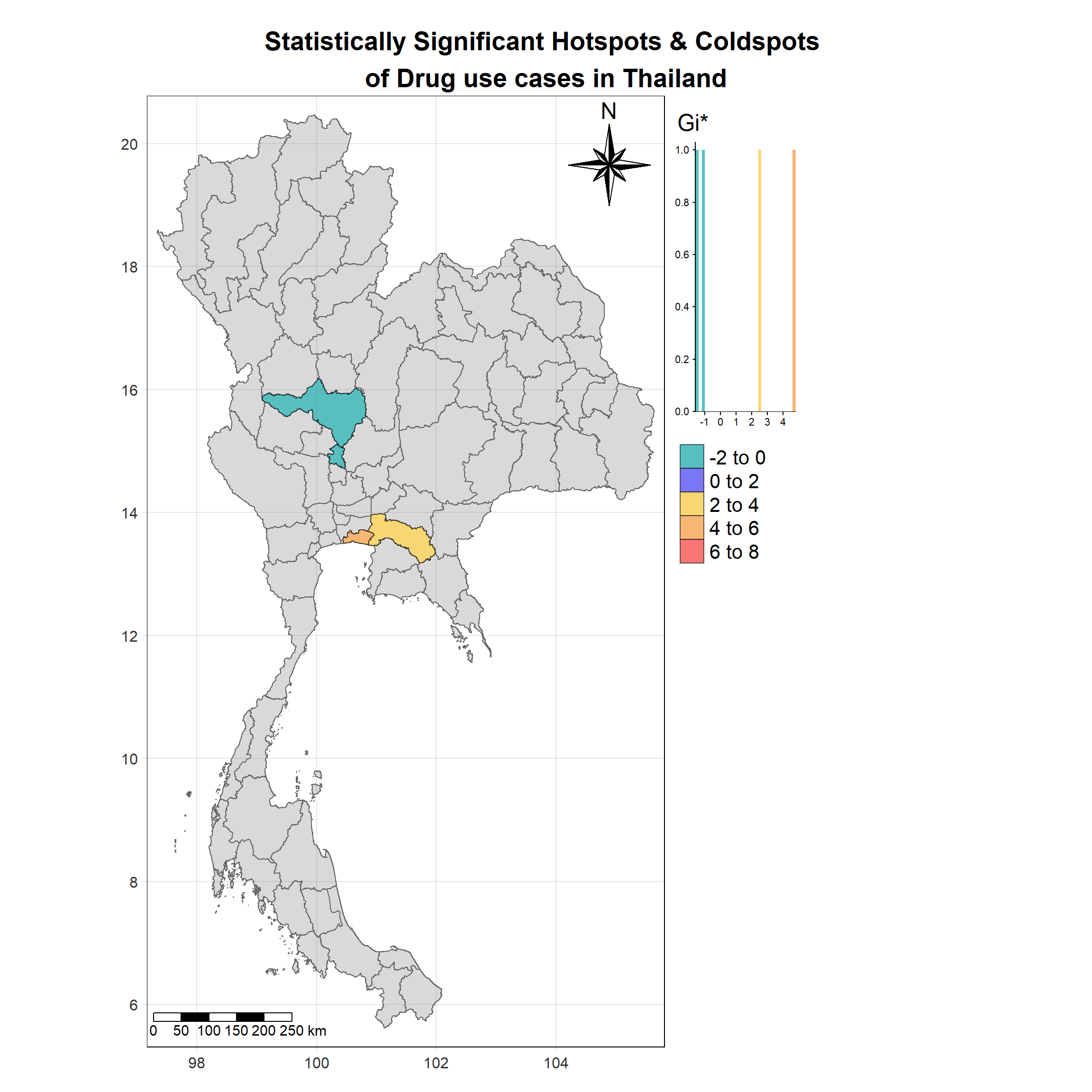

Top Hotspots and Coldspots Identification

We then identify the top hotspot provinces (with the highest positive gi_star values) and the top coldspot provinces (with the lowest negative gi_star values). It uses the filtered HCSA_<current_year>_sig dataset and arranges the values in descending and ascending order, respectively, to extract the top provinces.

# Get the top 3 hotspots (highest positive gi_star values)
top_hotspots <- HCSA_2020_sig %>%
  arrange(desc(gi_star)) %>%
  head(3) %>%
  pull(province_en)

# Get the top 3 cold spots (lowest negative gi_star values)
top_coldspots <- HCSA_2020_sig %>%
  filter(!(province_en %in% top_hotspots)) %>%
  arrange(gi_star) %>%
  head(3) %>%
  pull(province_en)

HCSA_top_hotspots <- HCSA_2020_sig %>% filter(province_en %in% top_hotspots)
HCSA_top_coldspots <- HCSA_2020_sig %>% filter(province_en %in% top_coldspots)

tm_shape(HCSA_2020) +
  tm_polygons() +
tm_shape(HCSA_top_hotspots)+
  tm_fill("gi_star", 
          palette = c("#f67774")) +
  tm_borders(col = "black", alpha = 0.6)+
  tm_text("province_en",auto.placement = T)+
  tm_layout(main.title = "Most Significant Hotspots of Drug use\n cases in Thailand",
            main.title.position = "center",
            main.title.size = 1.7,
            main.title.fontface = "bold",
            legend.show = FALSE,
            frame = TRUE) +
  tm_borders(alpha = 0.5) +
  tm_compass(type="8star", text.size = 1.5, size = 3, position=c("RIGHT", "TOP")) +
  tm_scale_bar(position=c("LEFT", "BOTTOM"), text.size=1.2) +
  tm_grid(labels.size = 1,alpha =0.2)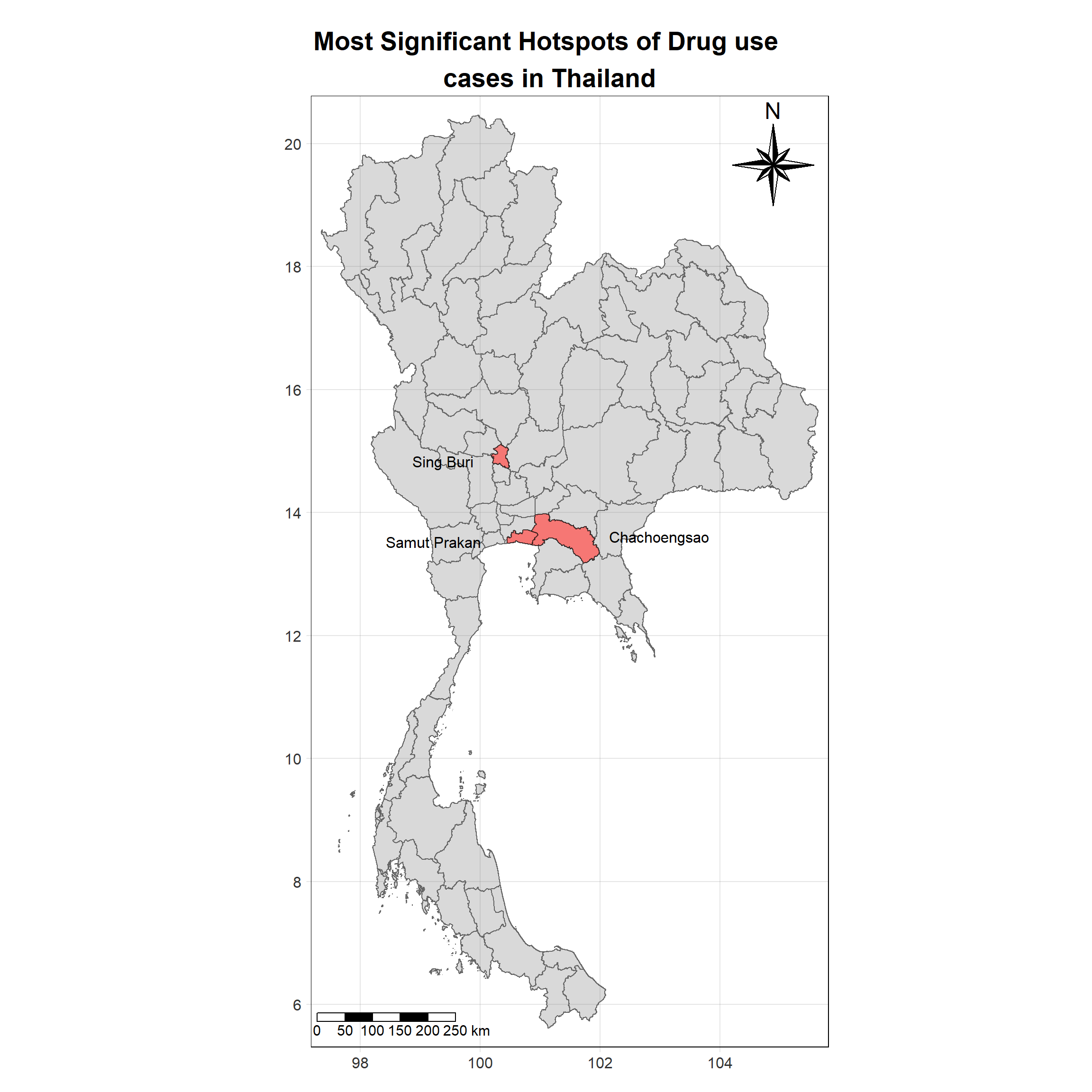

tm_shape(HCSA_2020) +
  tm_polygons() +
tm_shape(HCSA_top_coldspots)+
  tm_fill("gi_star", 
          palette = c("#57bfc0")) +
  tm_borders(col = "black", alpha = 0.6)+
  tm_text("province_en", auto.placement = T)+
  tm_layout(main.title = "Most Significant Coldspots of Drug use\n cases in Thailand",
            main.title.position = "center",
            main.title.size = 1.7,
            main.title.fontface = "bold",
            legend.show = FALSE,
            frame = TRUE) +
  tm_borders(alpha = 0.5) +
  tm_compass(type="8star", text.size = 1.5, size = 3, position=c("RIGHT", "TOP")) +
  tm_scale_bar(position=c("LEFT", "BOTTOM"), text.size=1.2) +
  tm_grid(labels.size = 1,alpha =0.2)

2021

Map of Hotspots & Coldspots of Drug Use Cases in Thailand

First we generate a map of Thailand for the current year, showing the hotspots and coldspots of drug use cases using Gi statistics. The fill color is determined by the gi_star column using a specified color palette, with a midpoint of 0 to distinguish between hotspots (positive Gi) and coldspots (negative Gi). The map also includes borders, a title, a compass, a scale bar, and a grid.

tm_shape(HCSA_2021)+
  tm_fill("gi_star", 
          palette = c("#57bfc0", "#7977f3","#f8d673","#f8b675","#f67774"),
          title = "Gi*",
          midpoint = 0) +
  tm_borders(col = "black", alpha = 0.6)+
  tm_layout(main.title = "2021 Hotspots & Coldspots of drug\n use cases in Thailand",
            main.title.position = "center",
            main.title.size = 1.7,
            main.title.fontface = "bold",
            legend.title.size = 1.8,
            legend.text.size = 1.3,
            legend.outside = TRUE,
            frame = TRUE) +
  tm_borders(alpha = 0.5) +
  tm_compass(type="8star", text.size = 1.5, size = 3, position=c("RIGHT", "TOP")) +
  tm_scale_bar(position=c("LEFT", "BOTTOM"), text.size=1.2) +
  tm_grid(labels.size = 1,alpha =0.2)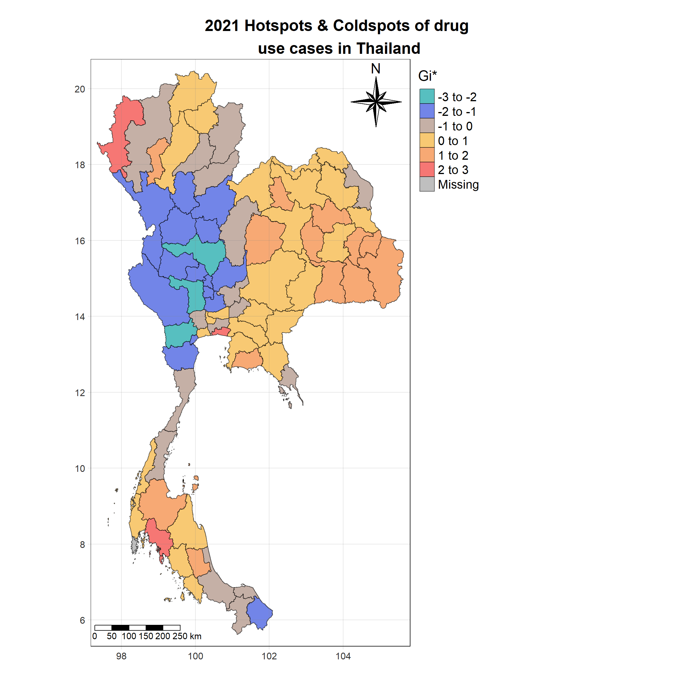

Map of Statistically Significant Hotspots & Coldspots of Drug Use Cases

We then create a map similar to the previous one but filters the data to only show provinces where the p_sim value is less than 0.05 (indicating statistically significant results). It visualizes the statistically significant hotspots and coldspots, with gi_star values categorized into specific intervals (breaks = c(-2, 0, 2, 4, 6, 8)), and includes a histogram in the legend for distribution reference.

HCSA_2021_sig <- HCSA_2021  %>%
  filter(p_sim < 0.05)

tm_shape(HCSA_2021) +
  tm_polygons() +
tm_shape(HCSA_2021_sig)+
  tm_fill("gi_star", 
          title = "Gi*",
          palette = c("#57bfc0", "#7977f3","#f8d673","#f8b675","#f67774"),
          breaks = c(-2, 0, 2, 4, 6, 8), 
          midpoint = 0,
          legend.hist = TRUE, 
          legend.is.portrait = TRUE,
          legend.hist.z = 0.1) +
  tm_borders(col = "black", alpha = 0.6)+
  tm_layout(main.title = "Statistically Significant Hotspots & Coldspots \nof Drug use cases in Thailand",
            main.title.position = "center",
            main.title.size = 1.7,
            main.title.fontface = "bold",
            legend.title.size = 1.8,
            legend.text.size = 1.3,
            legend.outside = TRUE,
            frame = TRUE) +
  tm_borders(alpha = 0.5) +
  tm_compass(type="8star", text.size = 1.5, size = 3, position=c("RIGHT", "TOP")) +
  tm_scale_bar(position=c("LEFT", "BOTTOM"), text.size=1.2) +
  tm_grid(labels.size = 1,alpha =0.2)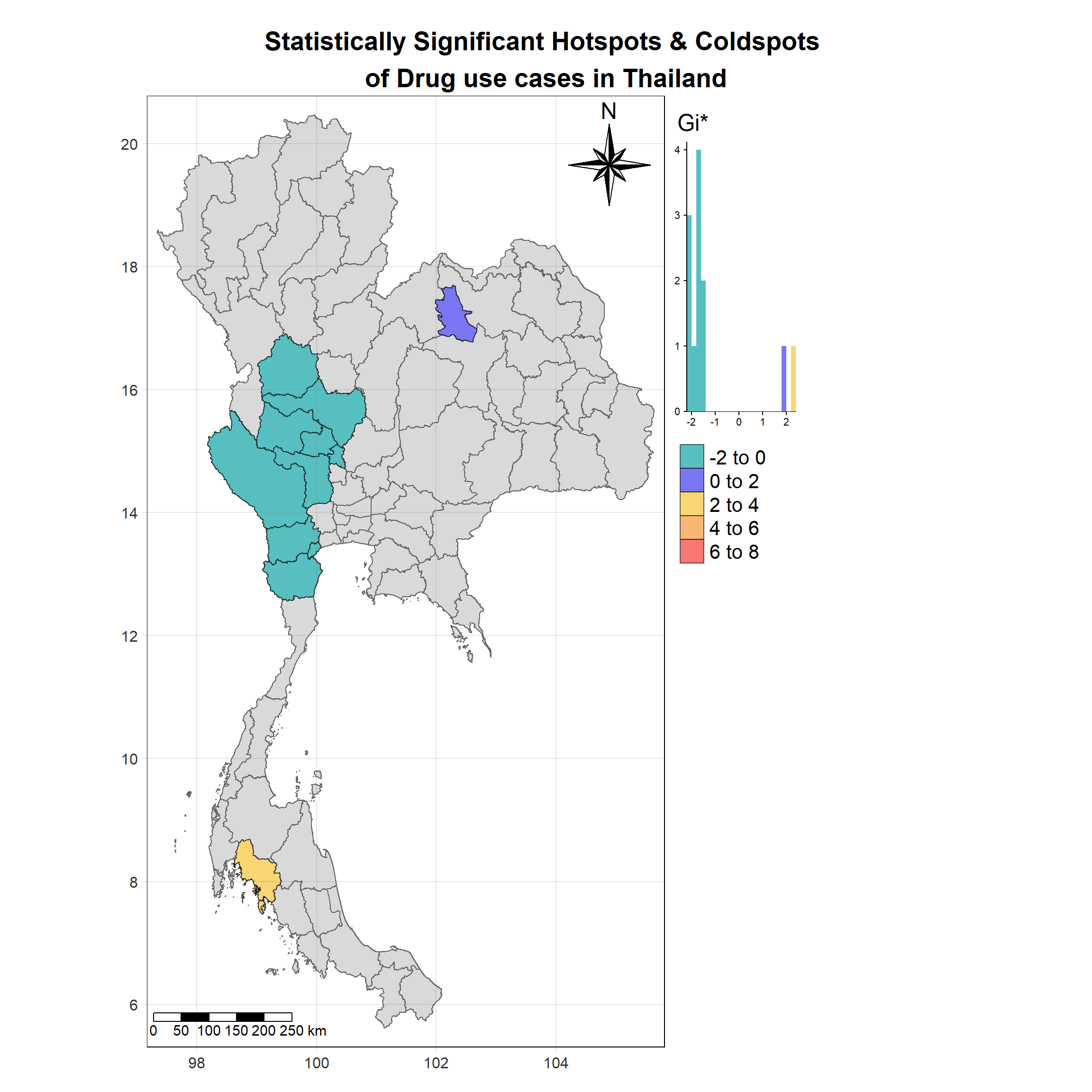

Top Hotspots and Coldspots Identification

We then identify the top hotspot provinces (with the highest positive gi_star values) and the top coldspot provinces (with the lowest negative gi_star values). It uses the filtered HCSA_<current_year>_sig dataset and arranges the values in descending and ascending order, respectively, to extract the top provinces.

# Get the top 3 hotspots (highest positive gi_star values)
top_hotspots <- HCSA_2021_sig %>%
  arrange(desc(gi_star)) %>%
  head(3) %>%
  pull(province_en)

# Get the top 3 cold spots (lowest negative gi_star values)
top_coldspots <- HCSA_2021_sig %>%
  filter(!(province_en %in% top_hotspots)) %>%
  arrange(gi_star) %>%
  head(3) %>%
  pull(province_en)

HCSA_top_hotspots <- HCSA_2021_sig %>% filter(province_en %in% top_hotspots)
HCSA_top_coldspots <- HCSA_2021_sig %>% filter(province_en %in% top_coldspots)

tm_shape(HCSA_2021) +
  tm_polygons() +
tm_shape(HCSA_top_hotspots)+
  tm_fill("gi_star", 
          palette = c("#f67774")) +
  tm_borders(col = "black", alpha = 0.6)+
  tm_text("province_en",auto.placement = T)+
  tm_layout(main.title = "Most Significant Hotspots of Drug use\n cases in Thailand",
            main.title.position = "center",
            main.title.size = 1.7,
            main.title.fontface = "bold",
            legend.show = FALSE,
            frame = TRUE) +
  tm_borders(alpha = 0.5) +
  tm_compass(type="8star", text.size = 1.5, size = 3, position=c("RIGHT", "TOP")) +
  tm_scale_bar(position=c("LEFT", "BOTTOM"), text.size=1.2) +
  tm_grid(labels.size = 1,alpha =0.2)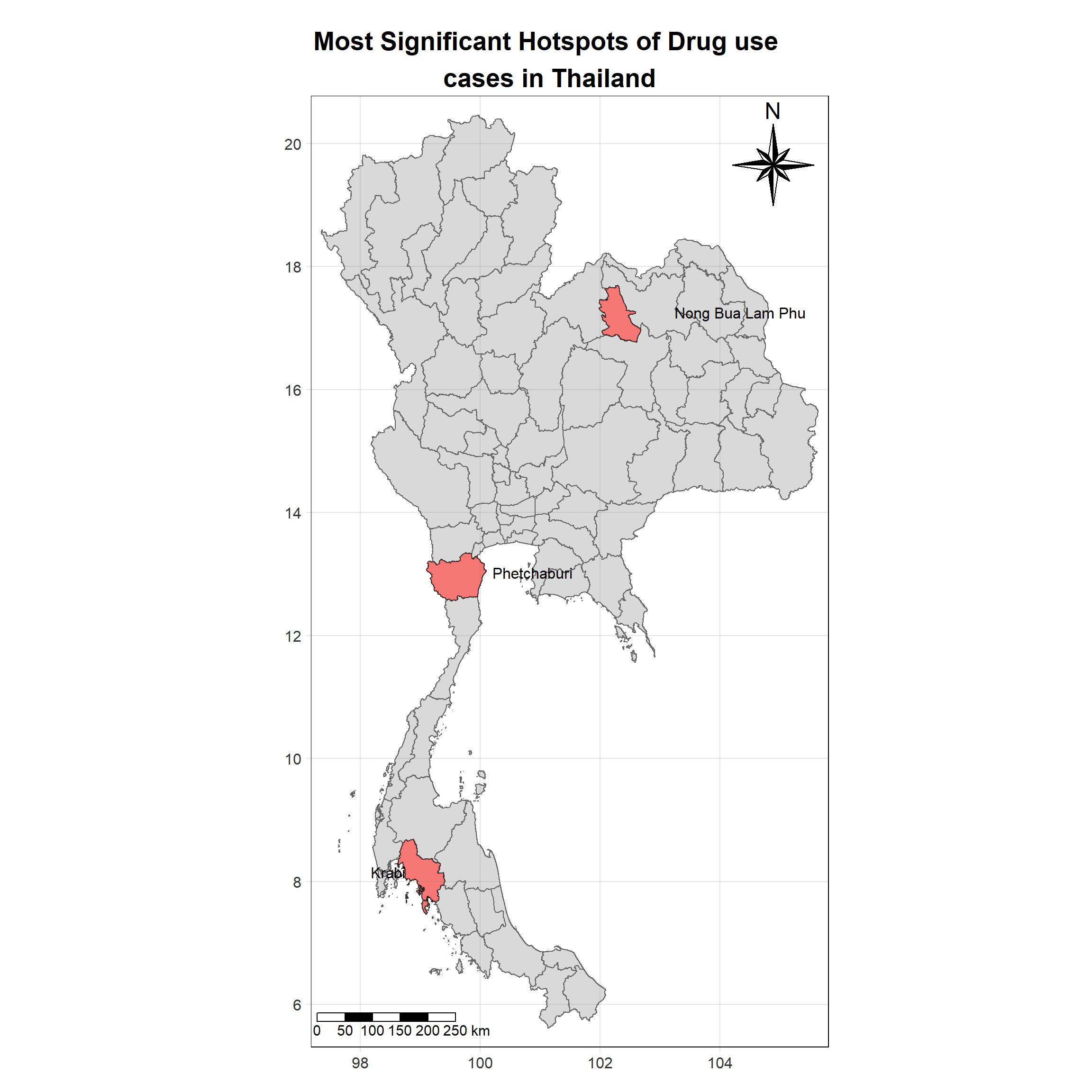

tm_shape(HCSA_2021) +
  tm_polygons() +
tm_shape(HCSA_top_coldspots)+
  tm_fill("gi_star", 
          palette = c("#57bfc0")) +
  tm_borders(col = "black", alpha = 0.6)+
  tm_text("province_en", auto.placement = T)+
  tm_layout(main.title = "Most Significant Coldspots of Drug use\n cases in Thailand",
            main.title.position = "center",
            main.title.size = 1.7,
            main.title.fontface = "bold",
            legend.show = FALSE,
            frame = TRUE) +
  tm_borders(alpha = 0.5) +
  tm_compass(type="8star", text.size = 1.5, size = 3, position=c("RIGHT", "TOP")) +
  tm_scale_bar(position=c("LEFT", "BOTTOM"), text.size=1.2) +
  tm_grid(labels.size = 1,alpha =0.2)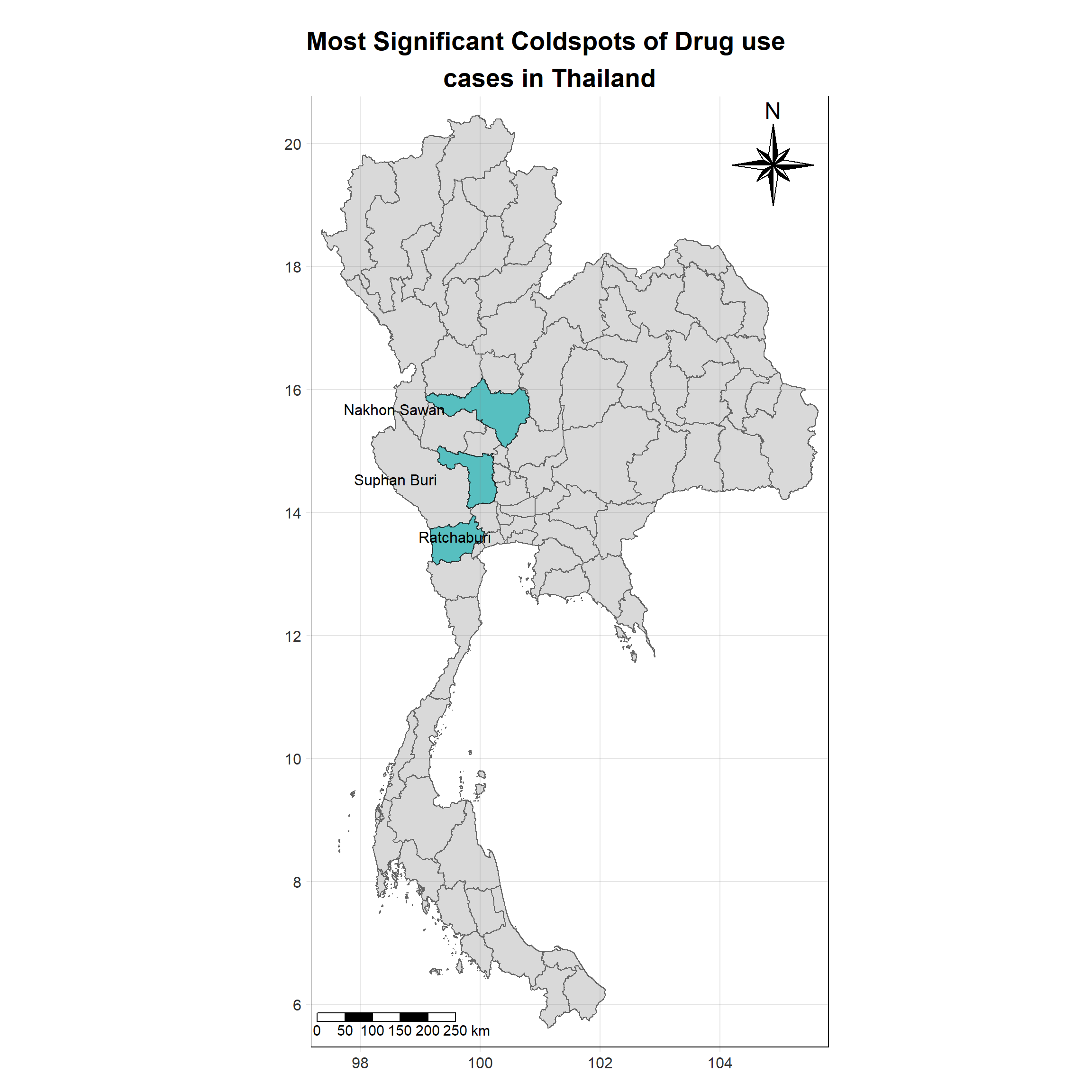

2022

Map of Hotspots & Coldspots of Drug Use Cases in Thailand

First we generate a map of Thailand for the current year, showing the hotspots and coldspots of drug use cases using Gi statistics. The fill color is determined by the gi_star column using a specified color palette, with a midpoint of 0 to distinguish between hotspots (positive Gi) and coldspots (negative Gi). The map also includes borders, a title, a compass, a scale bar, and a grid.

tm_shape(HCSA_2022)+
  tm_fill("gi_star", 
          palette = c("#57bfc0", "#7977f3","#f8d673","#f8b675","#f67774"),
          title = "Gi*",
          midpoint = 0) +
  tm_borders(col = "black", alpha = 0.6)+
  tm_layout(main.title = "2022 Hotspots & Coldspots of drug\n use cases in Thailand",
            main.title.position = "center",
            main.title.size = 1.7,
            main.title.fontface = "bold",
            legend.title.size = 1.8,
            legend.text.size = 1.3,
            legend.outside = TRUE,
            frame = TRUE) +
  tm_borders(alpha = 0.5) +
  tm_compass(type="8star", text.size = 1.5, size = 3, position=c("RIGHT", "TOP")) +
  tm_scale_bar(position=c("LEFT", "BOTTOM"), text.size=1.2) +
  tm_grid(labels.size = 1,alpha =0.2)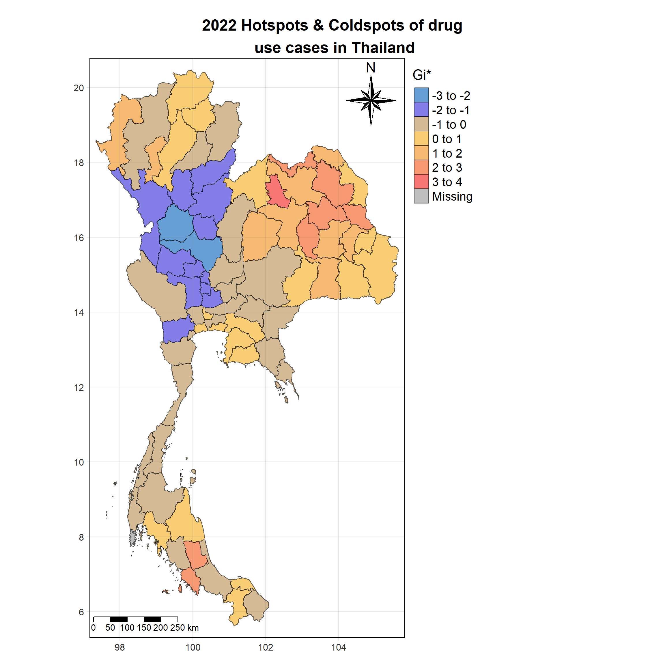

Map of Statistically Significant Hotspots & Coldspots of Drug Use Cases

We then create a map similar to the previous one but filters the data to only show provinces where the p_sim value is less than 0.05 (indicating statistically significant results). It visualizes the statistically significant hotspots and coldspots, with gi_star values categorized into specific intervals (breaks = c(-2, 0, 2, 4, 6, 8)), and includes a histogram in the legend for distribution reference.

HCSA_2022_sig <- HCSA_2022  %>%
  filter(p_sim < 0.05)

tm_shape(HCSA_2022) +
  tm_polygons() +
tm_shape(HCSA_2022_sig)+
  tm_fill("gi_star", 
          title = "Gi*",
          palette = c("#57bfc0", "#7977f3","#f8d673","#f8b675","#f67774"),
          breaks = c(-2, 0, 2, 4, 6, 8), 
          midpoint = 0,
          legend.hist = TRUE, 
          legend.is.portrait = TRUE,
          legend.hist.z = 0.1) +
  tm_borders(col = "black", alpha = 0.6)+
  tm_layout(main.title = "Statistically Significant Hotspots & Coldspots \nof Drug use cases in Thailand",
            main.title.position = "center",
            main.title.size = 1.7,
            main.title.fontface = "bold",
            legend.title.size = 1.8,
            legend.text.size = 1.3,
            legend.outside = TRUE,
            frame = TRUE) +
  tm_borders(alpha = 0.5) +
  tm_compass(type="8star", text.size = 1.5, size = 3, position=c("RIGHT", "TOP")) +
  tm_scale_bar(position=c("LEFT", "BOTTOM"), text.size=1.2) +
  tm_grid(labels.size = 1,alpha =0.2)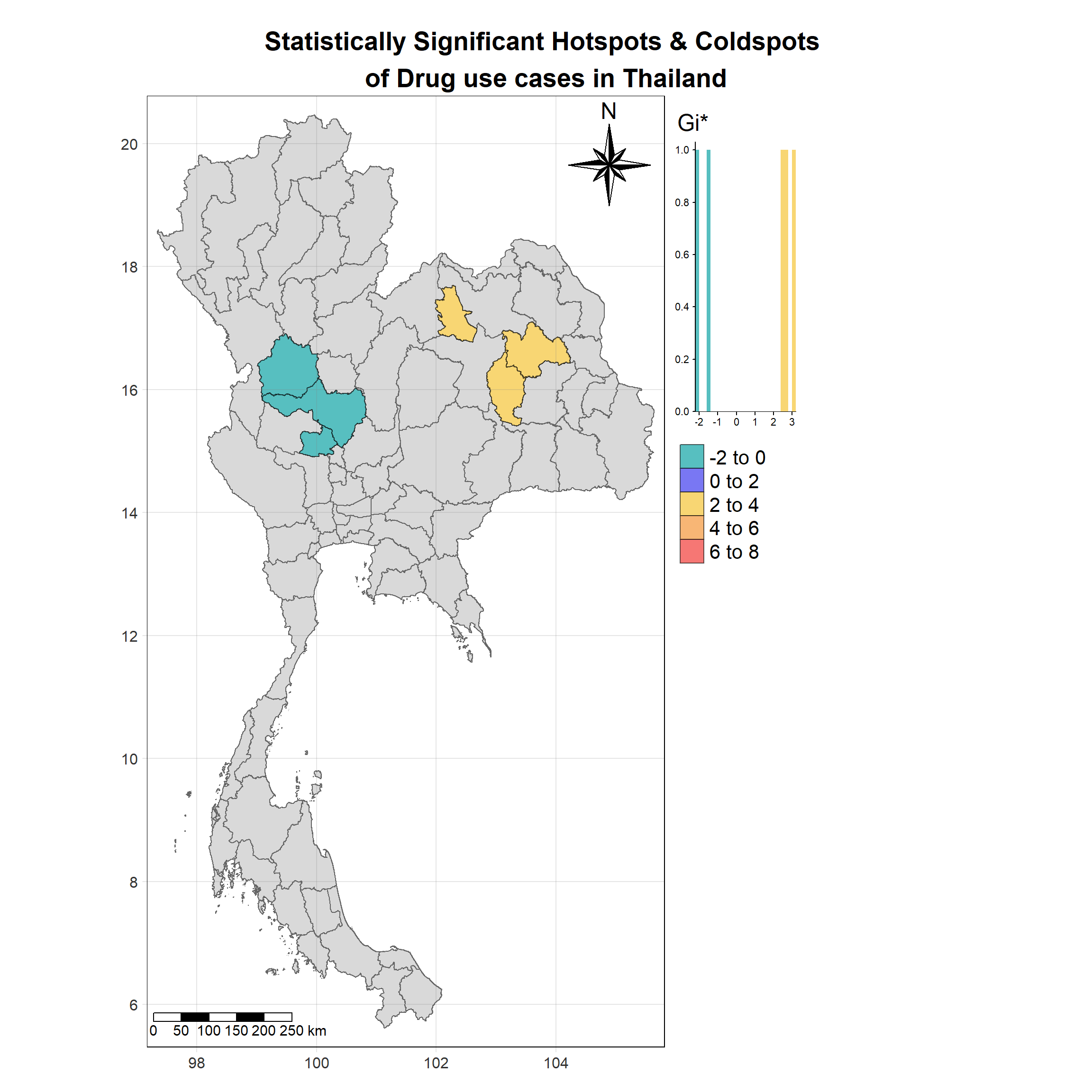

Top Hotspots and Coldspots Identification

We then identify the top hotspot provinces (with the highest positive gi_star values) and the top coldspot provinces (with the lowest negative gi_star values). It uses the filtered HCSA_<current_year>_sig dataset and arranges the values in descending and ascending order, respectively, to extract the top provinces.

# Get the top 3 hotspots (highest positive gi_star values)
top_hotspots <- HCSA_2022_sig %>%
  arrange(desc(gi_star)) %>%
  head(3) %>%
  pull(province_en)

# Get the top 3 cold spots (lowest negative gi_star values)
top_coldspots <- HCSA_2022_sig %>%
  filter(!(province_en %in% top_hotspots)) %>%
  arrange(gi_star) %>%
  head(3) %>%
  pull(province_en)

HCSA_top_hotspots <- HCSA_2022_sig %>% filter(province_en %in% top_hotspots)
HCSA_top_coldspots <- HCSA_2022_sig %>% filter(province_en %in% top_coldspots)

tm_shape(HCSA_2022) +
  tm_polygons() +
tm_shape(HCSA_top_hotspots)+
  tm_fill("gi_star", 
          palette = c("#f67774")) +
  tm_borders(col = "black", alpha = 0.6)+
  tm_text("province_en",auto.placement = T)+
  tm_layout(main.title = "Most Significant Hotspots of Drug use\n cases in Thailand",
            main.title.position = "center",
            main.title.size = 1.7,
            main.title.fontface = "bold",
            legend.show = FALSE,
            frame = TRUE) +
  tm_borders(alpha = 0.5) +
  tm_compass(type="8star", text.size = 1.5, size = 3, position=c("RIGHT", "TOP")) +
  tm_scale_bar(position=c("LEFT", "BOTTOM"), text.size=1.2) +
  tm_grid(labels.size = 1,alpha =0.2)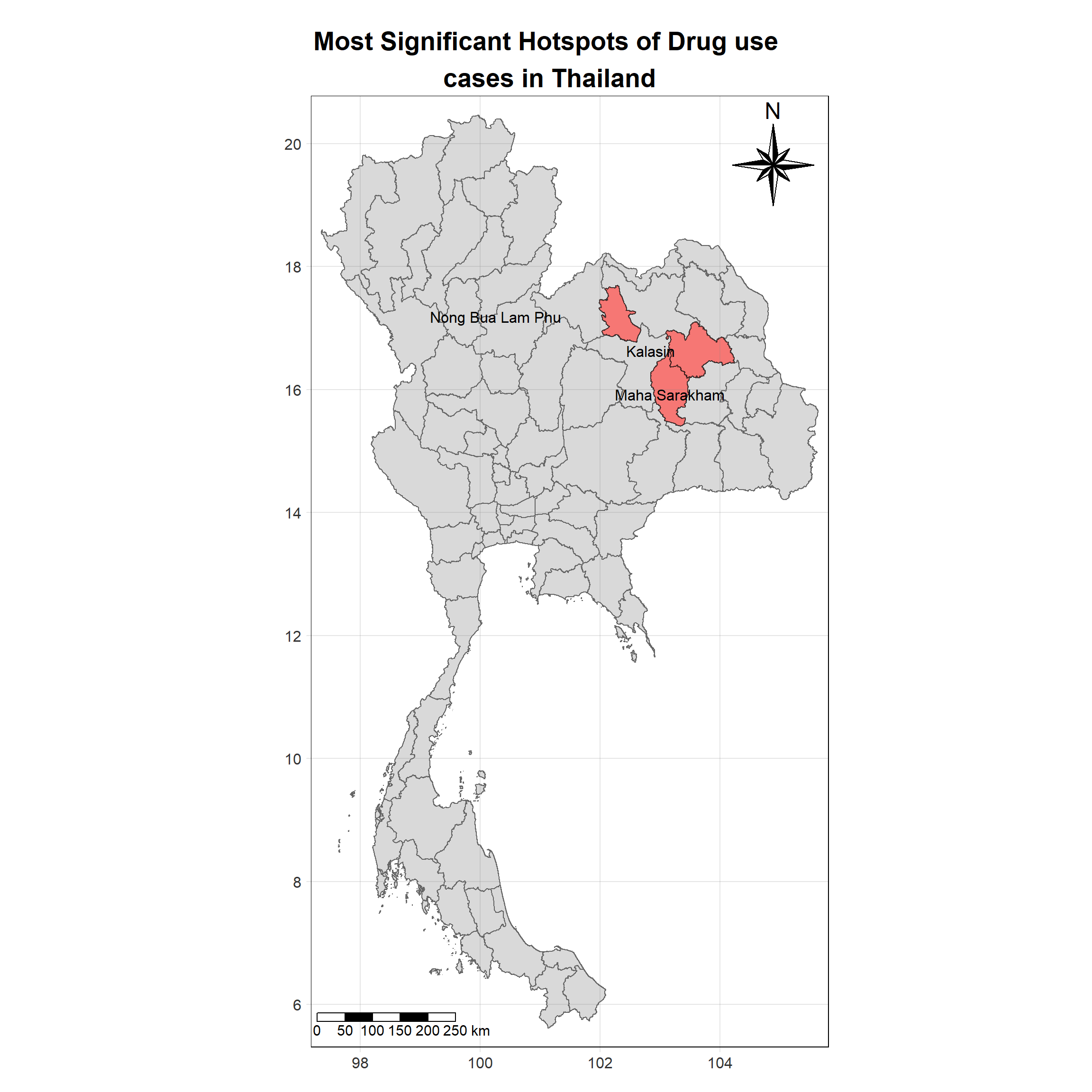

tm_shape(HCSA_2022) +
  tm_polygons() +
tm_shape(HCSA_top_coldspots)+
  tm_fill("gi_star", 
          palette = c("#57bfc0")) +
  tm_borders(col = "black", alpha = 0.6)+
  tm_text("province_en", auto.placement = T)+
  tm_layout(main.title = "Most Significant Coldspots of Drug use\n cases in Thailand",
            main.title.position = "center",
            main.title.size = 1.7,
            main.title.fontface = "bold",
            legend.show = FALSE,
            frame = TRUE) +
  tm_borders(alpha = 0.5) +
  tm_compass(type="8star", text.size = 1.5, size = 3, position=c("RIGHT", "TOP")) +
  tm_scale_bar(position=c("LEFT", "BOTTOM"), text.size=1.2) +
  tm_grid(labels.size = 1,alpha =0.2)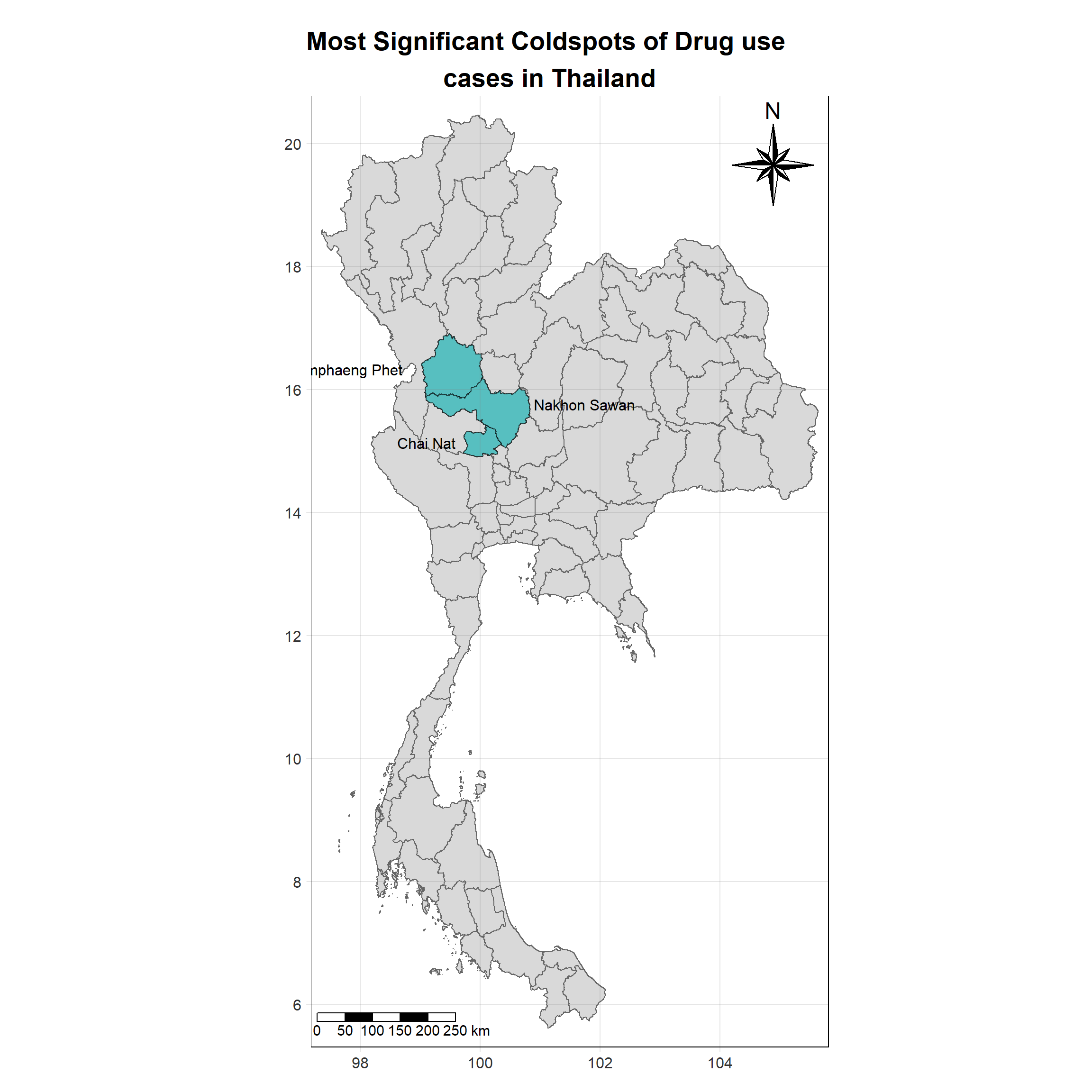

2.8.2 Discussion and Analysis

This spatial analysis enables better decision-making by highlighting areas that require focused attention. Identifying hotspots helps in targeting resources and interventions effectively, while coldspot areas provide insights into regions with fewer concerns. As demonstrated through the visualization, the Gi* analysis provides a clear and interpretable way to detect and map statistically significant clusters, facilitating data-driven policies and more informed public health strategies.

In general, the trend of drug use cases in Thailand from 2017 to 2022 generally aligns with the patterns revealed by the Local Indicator of Spatial Association (LISA) analysis. This suggests a consistent spatial clustering of drug-related incidents, where certain regions experience persistent high or low rates of drug use. The LISA analysis helps identify statistically significant hotspots and coldspots, reinforcing the spatial dependency observed in the distribution of these cases over the years.

2.9 Conclusion

The spatial analysis of drug-related cases in Thailand from 2017 to 2022, using Local Getis-Ord Gi and Local Indicator of Spatial Association (LISA), reveals distinct regional patterns that indicate both persistent hotspots and coldspots across different years. The northeastern region consistently exhibits High-High clusters, particularly in border provinces, suggesting an ongoing concentration of drug-related issues in those areas, highlighting them as persistent hotspots. These regions demand focused interventions to curb drug-related activities.

Conversely, the central and western regions show a contrasting trend with Low-Low clusters, signifying areas with stable, low drug-use rates, referred to as coldspots. The continued presence of these clusters across multiple years suggests the effectiveness of existing measures in maintaining lower levels of drug-related incidents in these regions. The spillover effects between neighboring regions, such as the emergence of Low-High and High-Low clusters, reflect transitional areas where drug-use trends might be shifting, requiring proactive monitoring and intervention strategies.

Overall, the combination of High-High and Low-Low clusters over the years demonstrates the evolving drug-use landscape in Thailand, necessitating a tailored approach to addressing both the hotspots and coldspots identified by spatial autocorrelation techniques like LISA and Local Getis-Ord Gi.

Key Recommendations

To effectively address the evolving landscape of drug use in Thailand, the authorities should adopt a data-driven, region-specific approach based on the spatial patterns observed in drug-related incidents from 2017 to 2022. Here are some key recommendations:

1. Focus on Persistent Hotspots: The northeastern region, particularly along the border provinces, consistently shows High-High clusters, indicating areas with a high concentration of drug-related cases. Thai authorities should prioritize these areas by intensifying law enforcement efforts, increasing surveillance, and providing targeted interventions. Coordinated cross-border efforts with neighboring countries might also help reduce the flow of drugs in these regions.

2. Strengthen Monitoring in Transitional Areas: The presence of High-Low and Low-High clusters in both the northeastern and central regions indicates areas where drug use trends may be shifting. Thai authorities should closely monitor these transitional areas to prevent the potential spillover of drug-related activities from high-incident to low-incident regions. Early intervention in these areas can help prevent further escalation of drug use.

3. Sustain Coldspots with Preventive Measures: In regions such as the central and western areas where Low-Low clusters are observed, authorities should continue supporting community-based preventive programs, education campaigns, and rehabilitation services. These measures have likely contributed to maintaining low levels of drug-related cases, and ensuring their sustainability will help preserve these coldspots.