pacman::p_load(sf, raster, spatstat, tmap, tidyverse, RColorBrewer, lubridate, ggplot2, parallel, sparr, magick)Take-home Exercise 1: Geospatial Analytics for Social Good: Application of Spatial and Spatio-temporal Point Patterns Analysis to discover the geographical distribution of Armed Conflict in Myanmar
Analysis
R
sf
tidyverse
raster
spatstat
tmap
tidyverse
1.1 Exercise Overview
Millions of people have their lives shattered by armed conflict – wars – every year.
Armed conflict has been on the rise since about 2012, after a decline in the 1990s and early 2000s. First came conflicts in Libya, Syria and Yemen, triggered by the 2011 Arab uprisings. Libya’s instability spilled south, helping set off a protracted crisis in the Sahel region. A fresh wave of major combat followed: the 2020 Azerbaijani-Armenian war over the Nagorno-Karabakh enclave, horrific fighting in Ethiopia’s northern Tigray region that began weeks later, the conflict prompted by the Myanmar army’s 2021 power grab and Russia’s 2022 assault on Ukraine. Add to those 2023’s devastation in Sudan and Gaza. Around the globe, more people are dying in fighting, being forced from their homes or in need of life-saving aid than in decades.
In this study, I will apply spatial point patterns analysis methods to discover the spatial and spatio-temporal distribution of armed conflict in Myanmar.
1.2 Data Acquisition
The data sets that we will be using are the following: - Armed conflict data of Myanmar between 2021-2024. This data can be downloaded from Armed Conflict Location & Event Data ACLED, an independent, impartial, international non-profit organization collecting data on violent conflict and protest in all countries and territories in the world, should be used. - The shapefile of the Myanmar State and Region Boundaries with Sub-regions. This data can be downloaded from Myanmar Information Management Unit, MIMU.
1.3 Getting Started
For this exercise, the following R packages will be used:
sf for handling geospatial data.
spatstat, a comprehensive package for point pattern analysis. We’ll use it to perform first- and second-order spatial point pattern analyses and to derive kernel density estimation (KDE) layers.
raster, a package for reading, writing, manipulating, and modeling gridded spatial data (rasters). We will use it to convert image outputs generated by spatstat into raster format.
tmap, a package for creating high-quality static and interactive maps, leveraging the Leaflet API for interactive visualizations.
tidyverse for performing data science tasks such as importing, wrangling and visualising data.
RColorBrewer for creating nice looking color palettes especially for thematic maps.
As readr, tidyr and dplyr are part of tidyverse package. The code chunk below will suffice to install and load the required packages in RStudio.
To install and load these packages into the R environment, we use the p_load function from the pacman package:
1.4 Importing Data into R
Next, we will import the ACLED-Southeast_Asia-Myanmar(1).csv file into the R environment and save it into an R dataframe called acled_sf. The task can be performed using the read_csv() function from the readr package, as shown below:
acled_sf <- read_csv("data/ACLED-Southeast_Asia-Myanmar(1).csv") %>%
  st_as_sf(coords = c(
    "longitude", "latitude"), crs = 4326) %>%
  st_transform(crs= 32647)%>%
  mutate(event_date = dmy(event_date)) %>%
  mutate(quarter = paste0(year, " Q", quarter(event_date)))
Notes
We used the mutate() function to ensure that the event_data column is in the right format of dmy(), while also creating a quarter column to represent the current
We can check the validity of the imported dataset, ensuring that it is in the right format with the st_crs() and summary() function:
st_crs(acled_sf)Coordinate Reference System:
User input: EPSG:32647
wkt:
PROJCRS["WGS 84 / UTM zone 47N",
BASEGEOGCRS["WGS 84",
ENSEMBLE["World Geodetic System 1984 ensemble",
MEMBER["World Geodetic System 1984 (Transit)"],
MEMBER["World Geodetic System 1984 (G730)"],
MEMBER["World Geodetic System 1984 (G873)"],
MEMBER["World Geodetic System 1984 (G1150)"],
MEMBER["World Geodetic System 1984 (G1674)"],
MEMBER["World Geodetic System 1984 (G1762)"],
MEMBER["World Geodetic System 1984 (G2139)"],
ELLIPSOID["WGS 84",6378137,298.257223563,
LENGTHUNIT["metre",1]],
ENSEMBLEACCURACY[2.0]],
PRIMEM["Greenwich",0,
ANGLEUNIT["degree",0.0174532925199433]],
ID["EPSG",4326]],
CONVERSION["UTM zone 47N",
METHOD["Transverse Mercator",
ID["EPSG",9807]],
PARAMETER["Latitude of natural origin",0,
ANGLEUNIT["degree",0.0174532925199433],
ID["EPSG",8801]],
PARAMETER["Longitude of natural origin",99,
ANGLEUNIT["degree",0.0174532925199433],
ID["EPSG",8802]],
PARAMETER["Scale factor at natural origin",0.9996,
SCALEUNIT["unity",1],
ID["EPSG",8805]],
PARAMETER["False easting",500000,
LENGTHUNIT["metre",1],
ID["EPSG",8806]],
PARAMETER["False northing",0,
LENGTHUNIT["metre",1],
ID["EPSG",8807]]],
CS[Cartesian,2],
AXIS["(E)",east,
ORDER[1],
LENGTHUNIT["metre",1]],
AXIS["(N)",north,
ORDER[2],
LENGTHUNIT["metre",1]],
USAGE[
SCOPE["Navigation and medium accuracy spatial referencing."],
AREA["Between 96°E and 102°E, northern hemisphere between equator and 84°N, onshore and offshore. China. Indonesia. Laos. Malaysia - West Malaysia. Mongolia. Myanmar (Burma). Russian Federation. Thailand."],
BBOX[0,96,84,102]],
ID["EPSG",32647]]summary(acled_sf) event_id_cnty event_date year time_precision
Length:42608 Min. :2021-01-01 Min. :2021 Min. :1.000
Class :character 1st Qu.:2022-01-10 1st Qu.:2022 1st Qu.:1.000
Mode :character Median :2022-10-13 Median :2022 Median :1.000
Mean :2022-10-29 Mean :2022 Mean :1.053
3rd Qu.:2023-08-29 3rd Qu.:2023 3rd Qu.:1.000
Max. :2024-06-30 Max. :2024 Max. :3.000
disorder_type event_type sub_event_type actor1
Length:42608 Length:42608 Length:42608 Length:42608
Class :character Class :character Class :character Class :character
Mode :character Mode :character Mode :character Mode :character
assoc_actor_1 inter1 actor2 assoc_actor_2
Length:42608 Min. :1.000 Length:42608 Length:42608
Class :character 1st Qu.:1.000 Class :character Class :character
Mode :character Median :1.000 Mode :character Mode :character
Mean :1.947
3rd Qu.:3.000
Max. :8.000
inter2 interaction civilian_targeting iso
Min. :0.000 Min. :10.00 Length:42608 Min. :104
1st Qu.:1.000 1st Qu.:13.00 Class :character 1st Qu.:104
Median :3.000 Median :17.00 Mode :character Median :104
Mean :3.597 Mean :18.86 Mean :104
3rd Qu.:7.000 3rd Qu.:17.00 3rd Qu.:104
Max. :8.000 Max. :80.00 Max. :104
region country admin1 admin2
Length:42608 Length:42608 Length:42608 Length:42608
Class :character Class :character Class :character Class :character
Mode :character Mode :character Mode :character Mode :character
admin3 location geo_precision source
Length:42608 Length:42608 Min. :1.000 Length:42608
Class :character Class :character 1st Qu.:1.000 Class :character
Mode :character Mode :character Median :1.000 Mode :character
Mean :1.495
3rd Qu.:2.000
Max. :3.000
source_scale notes fatalities tags
Length:42608 Length:42608 Min. : 0.00 Length:42608
Class :character Class :character 1st Qu.: 0.00 Class :character
Mode :character Mode :character Median : 0.00 Mode :character
Mean : 1.27
3rd Qu.: 1.00
Max. :201.00
timestamp geometry quarter
Min. :1.611e+09 POINT :42608 Length:42608
1st Qu.:1.702e+09 epsg:32647 : 0 Class :character
Median :1.714e+09 +proj=utm ...: 0 Mode :character
Mean :1.702e+09
3rd Qu.:1.719e+09
Max. :1.726e+09 We then import the boundaries and regions of Myanmar using the st_read() function to import the mmr_polbnda2_adm1_250k_mimu_1 shapefile into R as a simple feature data frame named regions_sf:
regions_sf <- st_read(dsn = "data/myanmar",
                layer = "mmr_polbnda2_adm1_250k_mimu_1")
Reading layer `mmr_polbnda2_adm1_250k_mimu_1' from data source
`C:\Users\blzll\OneDrive\Desktop\Y3S1\IS415\Quarto\IS415\Take-home_ex\data\myanmar'
using driver `ESRI Shapefile'
Simple feature collection with 18 features and 6 fields
Geometry type: MULTIPOLYGON
Dimension: XY
Bounding box: xmin: 92.1721 ymin: 9.696844 xmax: 101.17 ymax: 28.54554
Geodetic CRS: WGS 84regions_sf <- st_transform(regions_sf, crs = 32647)
Notes
The acled_sf and regions_sf data are being transformed to EPSG 32647, which corresponds to UTM Zone 47N. This CSR is fine for Myanmar. This consistency also ensures that the UTM zone transformation makes sense for the study area, and prevents any distortion in KDE results.
After importing the boundary and region data, we can check that what was imported is correct by checking the summary and plotting the views:
summary(regions_sf) OBJECTID ST ST_PCODE ST_RG
Min. : 1.00 Length:18 Length:18 Length:18
1st Qu.: 5.25 Class :character Class :character Class :character
Median : 9.50 Mode :character Mode :character Mode :character
Mean : 9.50
3rd Qu.:13.75
Max. :18.00
ST_MMR PCode_V geometry
Length:18 Min. :9.4 MULTIPOLYGON :18
Class :character 1st Qu.:9.4 epsg:32647 : 0
Mode :character Median :9.4 +proj=utm ...: 0
Mean :9.4
3rd Qu.:9.4
Max. :9.4 num_colors <- length(unique(regions_sf$ST))
colors <- brewer.pal(n = num_colors, name = "Set1")
tm_shape(regions_sf) +
tm_polygons(col = "ST", palette = colors) +
tm_text("ST", size = 0.9, col = "black", bg.color = "white",
just = c("center", "center"), xmod = 0, ymod = 0) +
tm_layout(main.title = "Region and Boundaries in Myanmar",
main.title.position = "center",
main.title.size = 1.6,
legend.outside = TRUE,
frame = TRUE) +
tm_legend(title = "Sub-regions")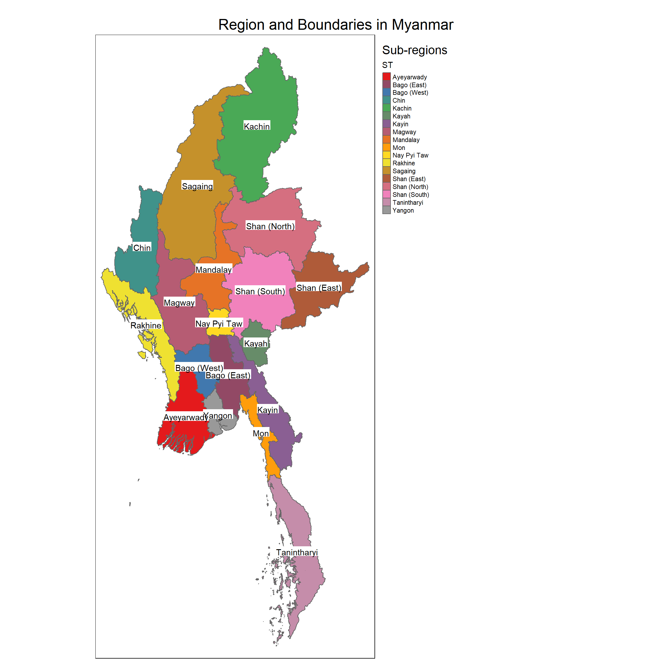
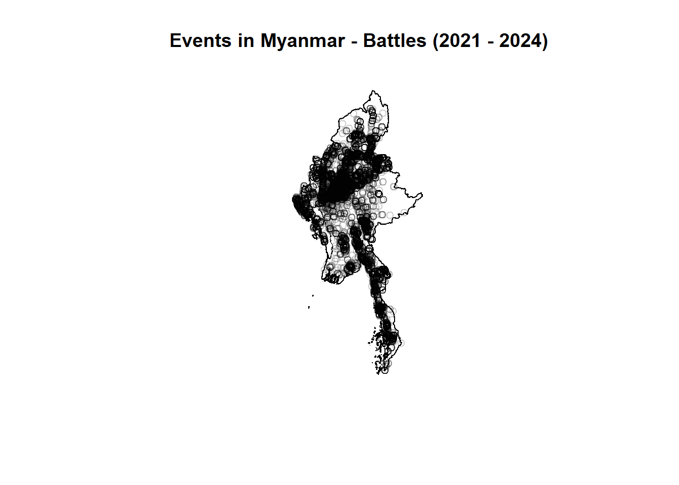
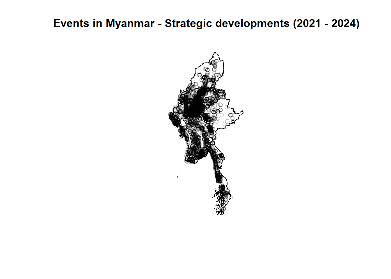
1.4.1 Focused Event Types
For the study, we focus on the following four event types from the ACLED dataset for Myanmar:
Battles
Strategic developments
Violence against civilians
Explosion/Remote violence
The study period spans from January 2021 to June 2024, broken down into quarterly intervals. We aim to visualize and analyze the spatial distribution of these armed conflict events in Myanmar.
The following function is used to generate spatial point pattern plots for each event type within the defined region throughout the stated time span:
# Function to create combined events object with owin object
plot_event_by_quarter <- function(event_data, event_name) {
  quarter_data_ppp <- as.ppp(st_coordinates(event_data), st_bbox(event_data))
  regions_owin <- as.owin(regions_sf)
  quarter_data_regions_ppp = quarter_data_ppp[regions_owin]

  plot(quarter_data_regions_ppp,
     main = paste("Events in Myanmar -", event_name, "(2021 - 2024)"),
     xlab = "Longitude", ylab = "Latitude")
}
# Get a list of unique quarters
events <- unique(acled_sf$event_type)
# Loop over each quarter and generate the plot
map(events, ~ {
event_data <- acled_sf %>% filter(event_type == .x)
plot_event_by_quarter(event_data, .x)
})


[[1]]
Symbol map with constant values
cols: #00000033

[[2]]
Symbol map with constant values
cols: #00000033

[[3]]
Symbol map with constant values
cols: #00000033

[[4]]
Symbol map with constant values
cols: #00000033
1.4.2 Storing key data
We will store key data sets intermittently to keep track of key data.
write_rds(acled_sf, "data/rds/acled_sf.rds")
write_rds(regions_sf, "data/rds/regions_sf.rds")
1.5 Determining KDE Layer
1.5.1 Choosing Sample Dataset
In this section, we focus on determining the appropriate Kernel Density Estimate (KDE) layer format for analyzing the spatial distribution of events across different quarters and event types. KDE is a fundamental tool for identifying patterns of spatial clustering and dispersion, providing a smooth surface that highlights areas of high and low event concentration. The selection of an appropriate bandwidth is crucial, as it influences the level of detail and accuracy in the density estimate. By standardizing the KDE layer format, we aim to ensure consistency and comparability throughout the analysis, particularly using the Violence against civilians event type as a reference for refining our approach.
Example <- "Violence against civilians"
acled_2021 <- acled_sf %>%
  filter(event_type == Example & year == 2021)
year_data <- as_Spatial(acled_2021)
regions <- as_Spatial(regions_sf)

year_data_sp <- as(year_data, "SpatialPoints")
regions_sp <- as(regions, "SpatialPolygons")

year_data_ppp <- as.ppp(st_coordinates(acled_2021), st_bbox(acled_2021))
year_data_ppp
Planar point pattern: 1877 points
window: rectangle = [-191409.1, 591875.9] x [1132472.1, 3042960.3] unitsany(duplicated(year_data_ppp))[1] TRUEAs there are duplicate points, we will use jittering to slightly displace the points so that overlapping points are separated on the map. The jitter parameter will slightly move each point by a small, random amount. This can help to visually separate points that are in the same space.
year_data_ppp_jit <- rjitter(year_data_ppp,
                             retry=TRUE,
                             nsim=1,
                             drop=TRUE)
any(duplicated(year_data_ppp_jit))
[1] FALSE1.5.2 Creating Owin Object
To confine analysis to a geographical area, convert the SpatialPolygon object to an owin object of spatstat:
regions_owin <- as.owin(regions_sf)

year_data_regions_ppp = year_data_ppp_jit[regions_owin]plot(year_data_regions_ppp)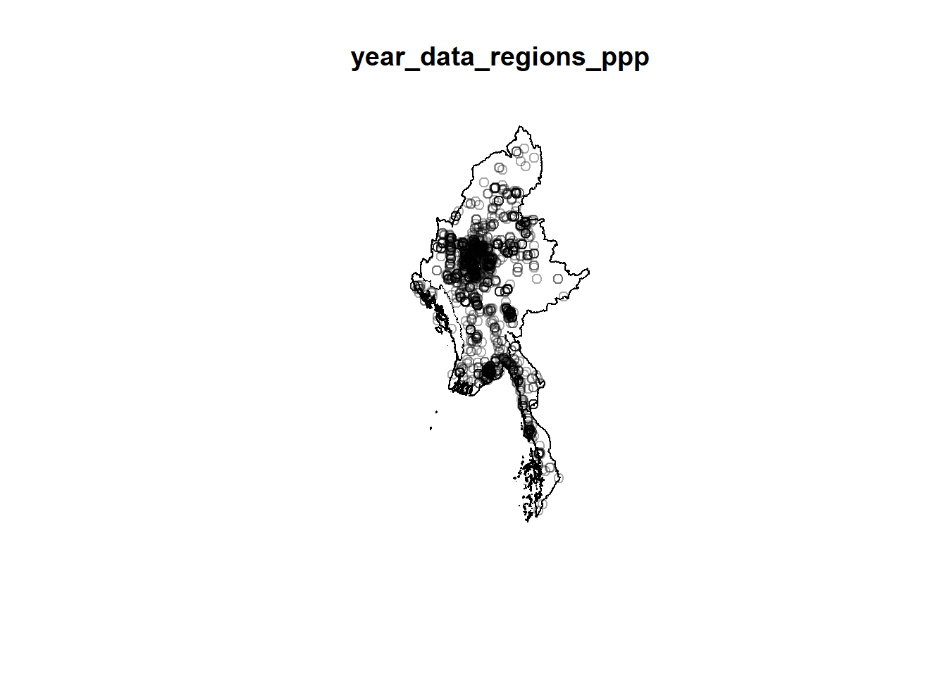
Due to the size of Myanmar, rescaling would need to be done:
year_data_regions_ppp.km <- rescale.ppp(year_data_regions_ppp, 50000, "km")1.5.3 Working With Different Automatic Bandwidth Methods
The density() function from the spatstat package computes the kernel density estimate for a given set of spatial point events, providing insights into the spatial distribution of those events.
bw.diggle(): This method selects the bandwidth (σ) by minimizing the mean-square error, as defined by Diggle (1985). The mean-square error measures the average squared difference between the estimated and actual values, aiming to reduce errors in the density estimate.bw.CvL(): Cronie and van Lieshout’s method selects the bandwidth by minimizing the discrepancy between the area of the observation window and the sum of reciprocal estimated intensity values at the event points. It balances the observed points and the space they occupy, capturing the underlying point process effectively.bw.scott(): Scott’s rule, a fast and computationally efficient method, calculates the bandwidth proportional to \((n^{-\frac{1}{d+4}})\), where (n) is the number of points and (d) the spatial dimensions. It typically produces a larger bandwidth and is ideal for detecting gradual trends.bw.ppl(): This method selects the bandwidth through likelihood cross-validation, maximizing the point process likelihood to provide the best-fitting model for the observed data, particularly when the goal is to optimize the likelihood of the given event distribution.
bw_CvL <- bw.CvL(year_data_regions_ppp.km)
bw_CvL
sigma
1.326217 bw_scott <- bw.scott(year_data_regions_ppp.km)
bw_scott sigma.x sigma.y
0.6923824 1.8282864 bw_ppl <- bw.ppl(year_data_regions_ppp.km)
bw_ppl sigma
0.1678648 bw_diggle <- bw.diggle(year_data_regions_ppp.km)
bw_diggle sigma
0.02286341 kde_diggle <- density(year_data_regions_ppp.km, bw_diggle)
kde_CvL <- density(year_data_regions_ppp.km, bw_CvL)
kde_scott <- density(year_data_regions_ppp.km, bw_scott)
kde_ppl <- density(year_data_regions_ppp.km, bw_ppl)
par(mar = c(2, 2, 2, 2),mfrow = c(2,2))
plot(kde_diggle, main = "kde_diggle")
plot(kde_CvL, main = "kde_CvL")
plot(kde_scott, main = "kde_scott")
plot(kde_ppl, main = "kde_ppl")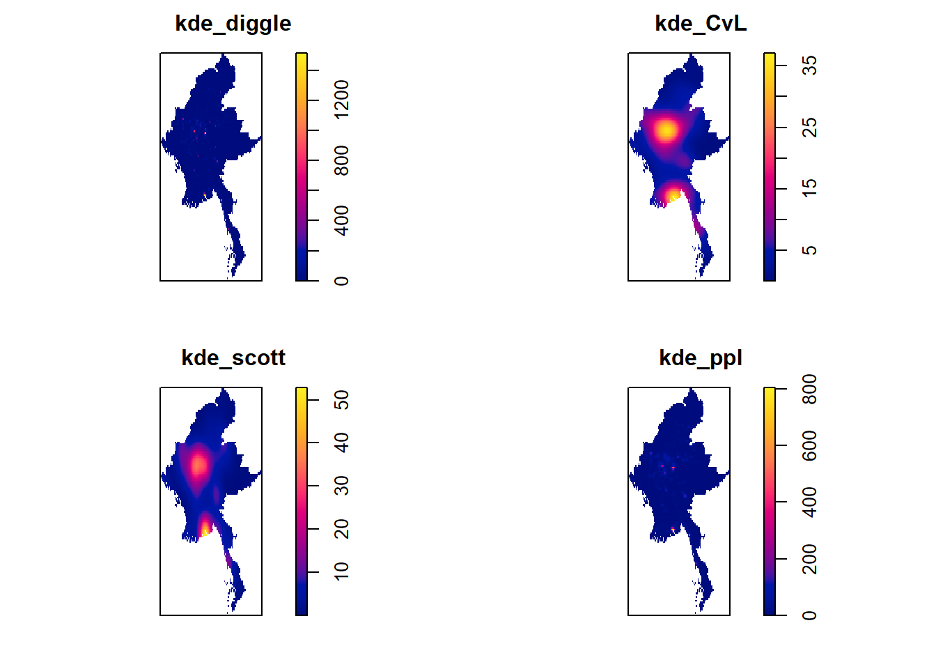
par(mar = c(2,2,2,2),mfrow = c(2,2))
hist(kde_diggle, main = "kde_diggle")
hist(kde_CvL, main = "kde_CvL")
hist(kde_scott, main = "kde_scott")
hist(kde_ppl, main = "kde_ppl")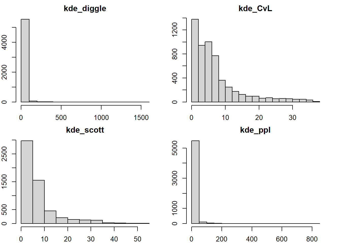
Reflection
Bandwidth Selection Comparison for KDE:
kde_diggle: The sharp peak at the beginning indicates that the Diggle method for bandwidth selection has identified a concentrated cluster of points in the initial bin. The remaining bins show little to no concentration, suggesting a significant level of spatial clustering in one specific area within the observation window. This method may highlight a localized, high-intensity clustering effect.
kde_CvL: The left-skewed, more balanced distribution suggests that the CvL method is identifying a broader range of spatial concentrations. However, the smaller bin sizes smooth out finer details, which could mask important aspects of the point pattern. This method provides a more generalized view of the distribution but at the cost of losing granular insights.
kde_scott: The wider range of values and the absence of a sharp peak, compared to kde_diggle, indicates that the Scott method is capturing both highly dense clusters and moderately concentrated areas. This makes it more suitable for capturing variations in spatial concentration across different regions.
kde_ppl: Similar to the Diggle method, kde_ppl shows a sharp peak, suggesting the presence of a high concentration of points in a specific region. This points to a localized cluster, but with a similar potential risk of missing broader patterns in the dataset.
dse_diggle <- density(year_data_regions_ppp.km, bw_diggle, se=TRUE)$SE
dse_CvL <- density(year_data_regions_ppp.km, bw_CvL, se=TRUE)$SE
dse_scott <- density(year_data_regions_ppp.km, bw_scott, se=TRUE)$SE
dse_ppl <- density(year_data_regions_ppp.km, bw_ppl, se=TRUE)$SEpar(mar = c(2,2,2,2),mfrow = c(2,2))
plot(dse_diggle,main = "standard error_diggle")
plot(dse_CvL,main = "standard error_CvL")
plot(dse_scott,main = "standard error_scott")
plot(dse_ppl,main = "standard error_ppl")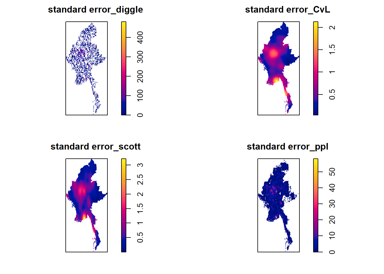
Reflection
Consideration of Standard Error:
While the standard error (SE) of the density estimate provides valuable insight into the uncertainty associated with each density estimate, it is not the primary focus of this analysis. The shape of the density estimate, rather than its absolute value, is more critical when analyzing spatial patterns. Consequently, the SE was not used as a key criterion for bandwidth selection in this analysis.
Consideration of Standard Error: While the standard error (SE) of the density estimate provides valuable insight into the uncertainty associated with each density estimate, it is not the primary focus of this analysis. The shape of the density estimate, rather than its absolute value, is more critical when analyzing spatial patterns. Consequently, the SE was not used as a key criterion for bandwidth selection in this analysis.
1.5.4 Final Bandwidth Selection
Upon the exploration of various fixed bandwidth selection methods for computing KDE vales, and subsequent plotting of the respective KDE estimates, their distributions and associated standard errors, we will now select the KDE bandwidth to be used in our analysis.
We landed on the bw_scott method for further analysis. This is because:
bw_scottmethod provides a pair of bandwidth values for each coordinate axis. This allows it to capture the different levels of spatial clustering in each direction more accurately.bw_scottmethod capture the balance between bias and variance the best among all methods. If the bandwidth is too small, the estimate may be too skewed (high variance). The distribution histograms of KDE layers usingbw_diggleandbw_ppltend to indicate such nature. On the other hand, if the bandwidth is too large, the estimate may be over smoothed, missing crucial elements of the point pattern (high bias). This is what we observed in the distribution histogram of KDE layer usingbw_CvL.
Since we have chosen to use bw_scott method, now we will plot the KDE layer using this method for further analysis.
1.5.4.1 Working With Different Kernel Methods
Beyond the Gaussian kernel, three other kernels can be used to compute KDE: - Epanechnikov - Quartic - Disc
par(mfrow=c(2,2), mar=c(1, 1, 1, 1), cex=0.5)
plot(density(year_data_regions_ppp.km,
             sigma=bw_scott,
             edge=TRUE,
             kernel="gaussian"),
     main="Gaussian")
plot(density(year_data_regions_ppp.km,
             sigma=bw_scott,
             edge=TRUE,
             kernel="epanechnikov"),
     main="Epanechnikov")
plot(density(year_data_regions_ppp.km,
             sigma=bw_scott,
             edge=TRUE,
             kernel="quartic"),
     main="Quartic")
plot(density(year_data_regions_ppp.km,
             sigma=bw_scott,
             edge=TRUE,
             kernel="disc"),
     main="Disc")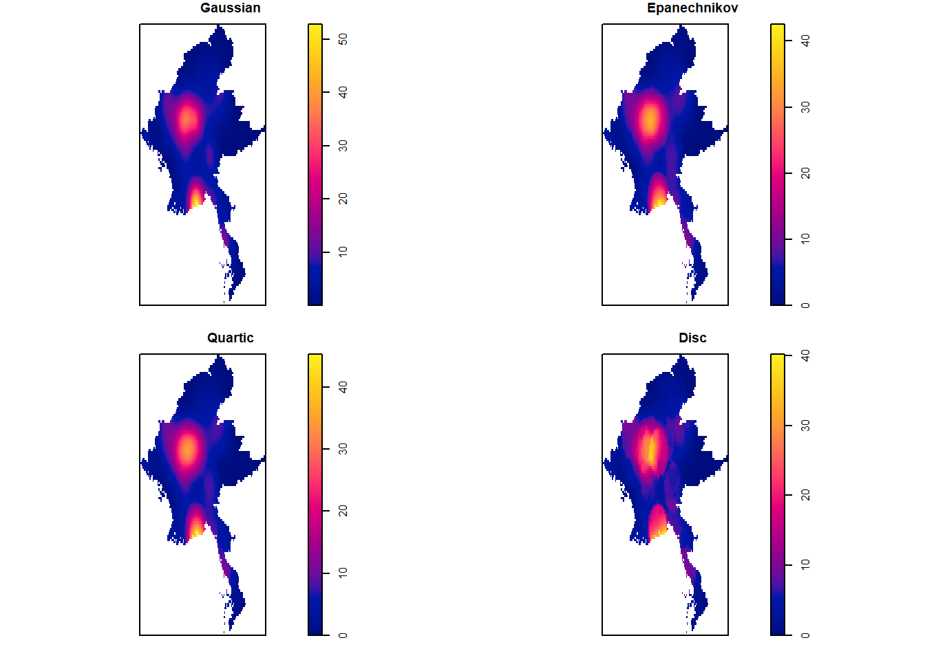
Reflection
Upon comparing the outputs of different kernel functions (Gaussian, Epanechnikov, Quartic, Disc), we observed that the resulting density estimates were very similar across all kernels. Given the minimal variation, the choice of kernel is not critical for this particular analysis.
We opted for the Gaussian kernel as it is widely used in kernel density estimation and tends to produce smooth, continuous estimates. Its flexibility in capturing both sharp peaks and gradual trends makes it a reasonable default choice, especially when the differences between kernels are negligible, as seen here.
kde_fixed_scott <- density(year_data_regions_ppp.km, bw_scott)
plot(kde_fixed_scott,main = "Fixed bandwidth KDE (Using bw_scott)")
contour(kde_fixed_scott, add=TRUE)
However, upon visual inspection, there are signs of a certain degree of over-smoothing when directly applying the bandwidth provided by the bw_scott method. While automatic bandwidth selection methods offer a useful starting point, further fine-tuning is often necessary to ensure the accuracy of the KDE plot.
To address the over-smoothing, we will apply a “rule of thumb” adjustment by dividing the bandwidth value by 2. This reduction in bandwidth size will help minimize the over-smoothing effect and enhance the precision of the spatial point pattern analysis.
kde_year_data_regions_fixed_scott <- density(year_data_regions_ppp.km, bw_scott/2)
kde_year_data_regions_adaptive <- adaptive.density(year_data_regions_ppp.km, method="kernel")

par(mfrow=c(1,2))
plot(kde_year_data_regions_fixed_scott, main = "Fixed Bandwidth (bw_scott)")
plot(kde_year_data_regions_adaptive, main = "Adaptive Bandwidth")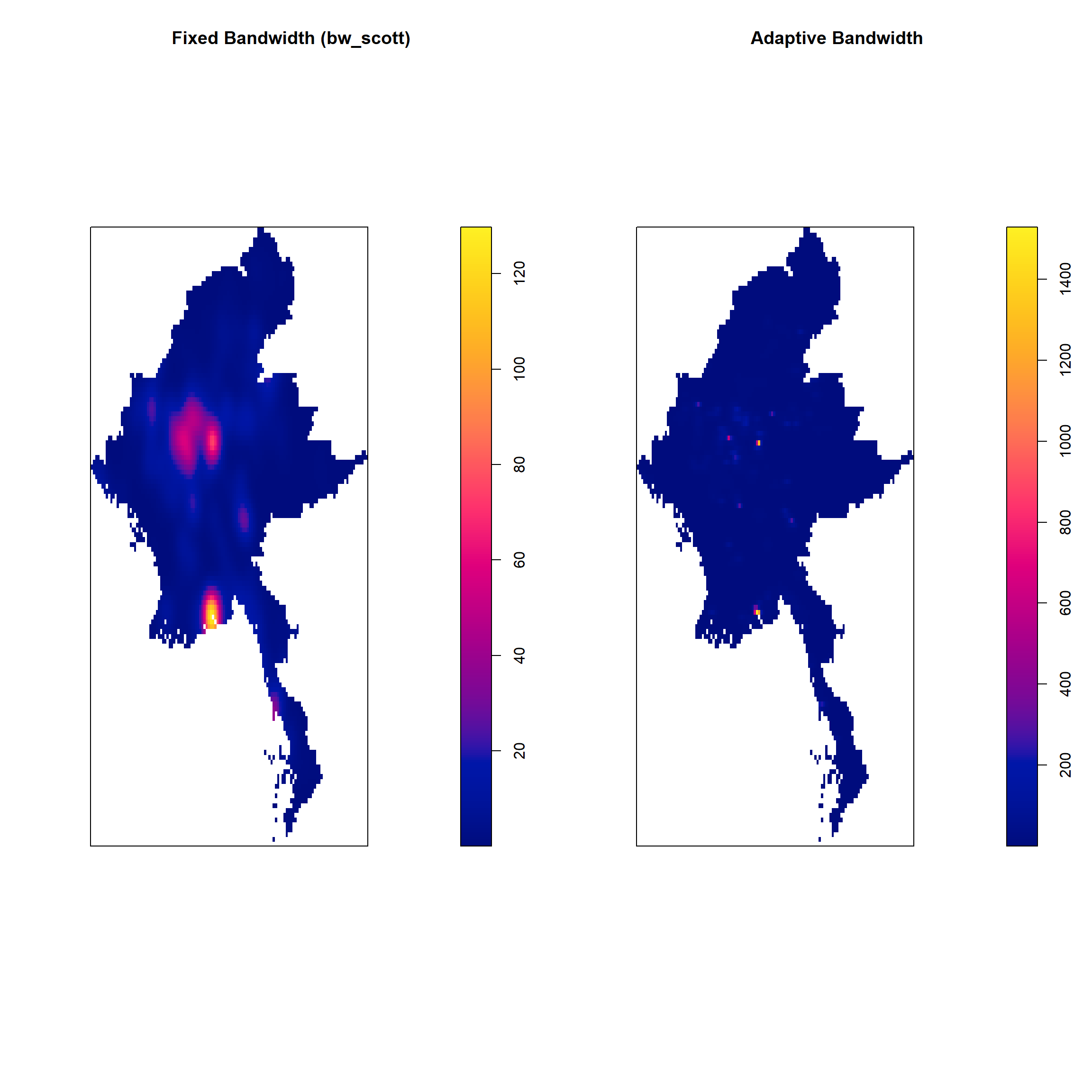
1.5.4.2 Plotting Interactive KDE Maps
raster_kde_fixed_scott <- raster(kde_year_data_regions_fixed_scott)
raster_kde_adaptive_kernel <- raster(kde_year_data_regions_adaptive)

# Set the correct CRS for the raster (EPSG:32647)
projection(raster_kde_fixed_scott) <- CRS("+init=EPSG:32647 +units=km")
projection(raster_kde_adaptive_kernel) <- CRS("+init=EPSG:32647 +units=km")tmap_mode('view')
kde_fixed_scott <- tm_basemap(server = "OpenStreetMap") +
tm_basemap(server = "Esri.WorldImagery") +
tm_shape(raster_kde_fixed_scott) +
tm_raster("layer",
n = 10,
title = "KDE_Fixed_scott",
alpha = 0.6,
palette = c("#fafac3","#fd953b","#f02a75","#b62385","#021c9e")) +
tm_shape(regions_sf) + # Transform only for visualization
tm_polygons(alpha=0.1, id="ST_PCODE") +
tmap_options(check.and.fix = TRUE)
kde_adaptive_kernel <- tm_basemap(server = "OpenStreetMap") +
tm_basemap(server = "Esri.WorldImagery") +
tm_shape(raster_kde_adaptive_kernel) +
tm_raster("layer",
n = 7,
title = "KDE_Adaptive_Kernel",
style = "pretty",
alpha = 0.6,
palette = c("#fafac3","#fd953b","#f02a75","#b62385","#021c9e")) +
tm_shape(regions_sf) + # Transform only for visualization
tm_polygons(alpha=0.1, id="ST_PCODE") +
tmap_options(check.and.fix = TRUE)
tmap_arrange(kde_fixed_scott, kde_adaptive_kernel, ncol=1, nrow=2, sync = TRUE)
Reflection
After comparing the two approaches for kernel density estimation, Fixed Bandwidth using bw_scott/2 and Adaptive Bandwidth, we observed that the fixed bandwidth method provides a more stable and interpretable result across the observation window. While adaptive bandwidth is designed to adjust to local point densities and capture finer details, it can sometimes introduce unnecessary complexity and overfit the density estimate, especially in areas with sparse data.
Given the goals of our analysis, which emphasize consistency and smoothness over high local sensitivity, the Fixed Bandwidth approach strikes a better balance between capturing spatial trends and avoiding over-complication.
1.5.4.3 Viewing Quarterly KDE Maps
Year 2021
Quarter 1
Example <- "Explosions/Remote violence"
my_2021_Q1 <- acled_sf  %>%
  filter(event_type == Example & quarter == "2021 Q1")

write_rds(my_2021_Q1, "data/rds/my_2021_Q1_ER_quarter_data_regions_sf.rds")

quarter_data <- as_Spatial(my_2021_Q1)
quarter_data_sp <- as(quarter_data, "SpatialPoints")
quarter_data_ppp <- as.ppp(st_coordinates(my_2021_Q1), st_bbox(my_2021_Q1))

quarter_data_ppp_jit <- rjitter(quarter_data_ppp,
                             retry=TRUE,
                             nsim=1,
                             drop=TRUE)
my_2021_Q1_ER_quarter_data_regions_ppp = quarter_data_ppp_jit[regions_owin]
quarter_data_regions_ppp.km <- rescale.ppp(my_2021_Q1_ER_quarter_data_regions_ppp, 50000, "km")
bw_scott <- bw.scott(quarter_data_regions_ppp.km)
plot(density(quarter_data_regions_ppp.km,
sigma=bw_scott/2,
edge=TRUE,
kernel="gaussian"),
main = "2021 Q1 - Explosion/Remote violence")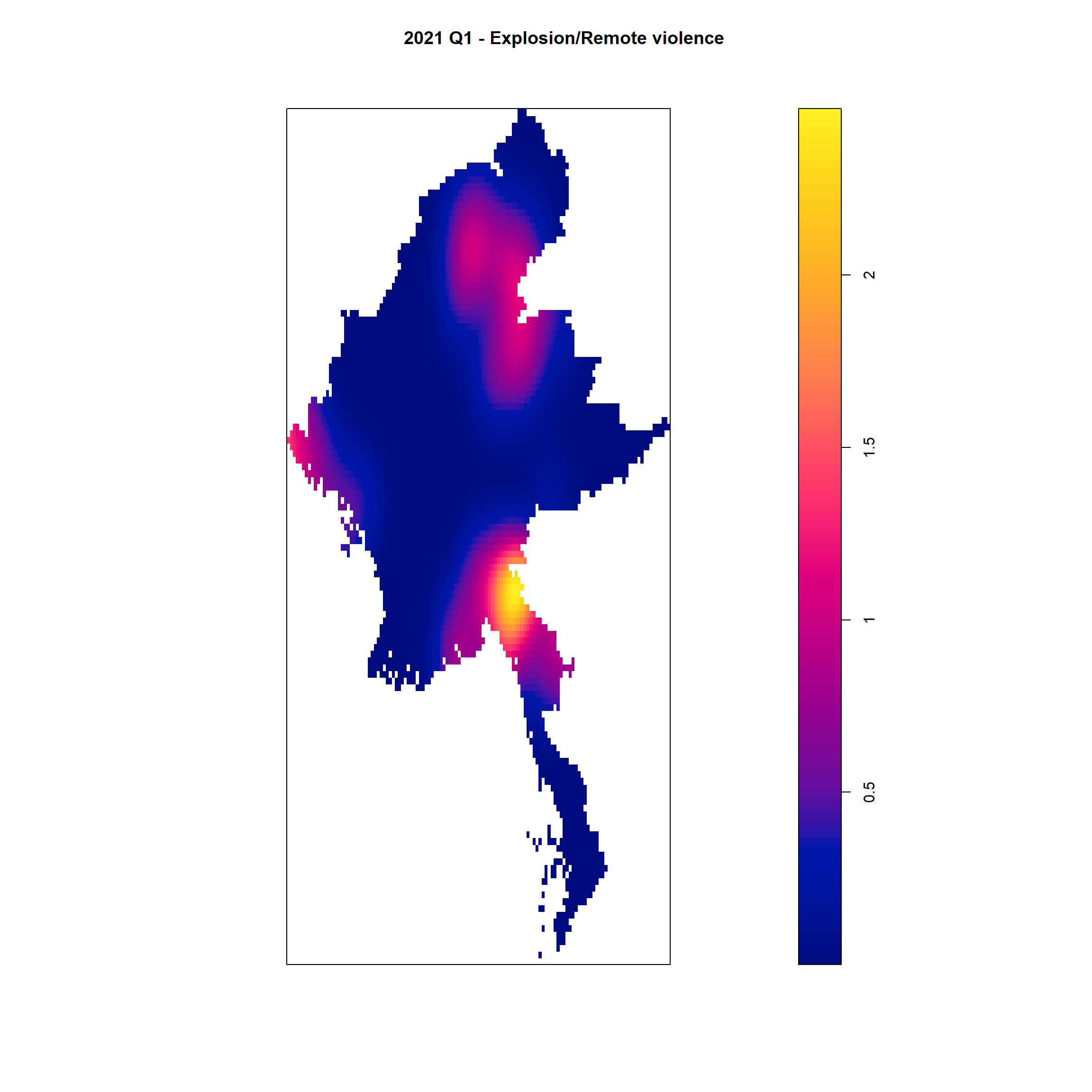
Example <- "Strategic developments"
my_2021_Q1 <- acled_sf  %>%
  filter(event_type == Example & quarter == "2021 Q1")

write_rds(my_2021_Q1, "data/rds/my_2021_Q1_SD_quarter_data_regions_sf.rds")

quarter_data <- as_Spatial(my_2021_Q1)
quarter_data_sp <- as(quarter_data, "SpatialPoints")
quarter_data_ppp <- as.ppp(st_coordinates(my_2021_Q1), st_bbox(my_2021_Q1))

quarter_data_ppp_jit <- rjitter(quarter_data_ppp,
                             retry=TRUE,
                             nsim=1,
                             drop=TRUE)
my_2021_Q1_SD_quarter_data_regions_ppp = quarter_data_ppp_jit[regions_owin]
quarter_data_regions_ppp.km <- rescale.ppp(my_2021_Q1_SD_quarter_data_regions_ppp , 50000, "km")
bw_scott <- bw.scott(quarter_data_regions_ppp.km)
plot(density(quarter_data_regions_ppp.km,
sigma=bw_scott/2,
edge=TRUE,
kernel="gaussian"),
main = "2021 Q1 - Strategic developments")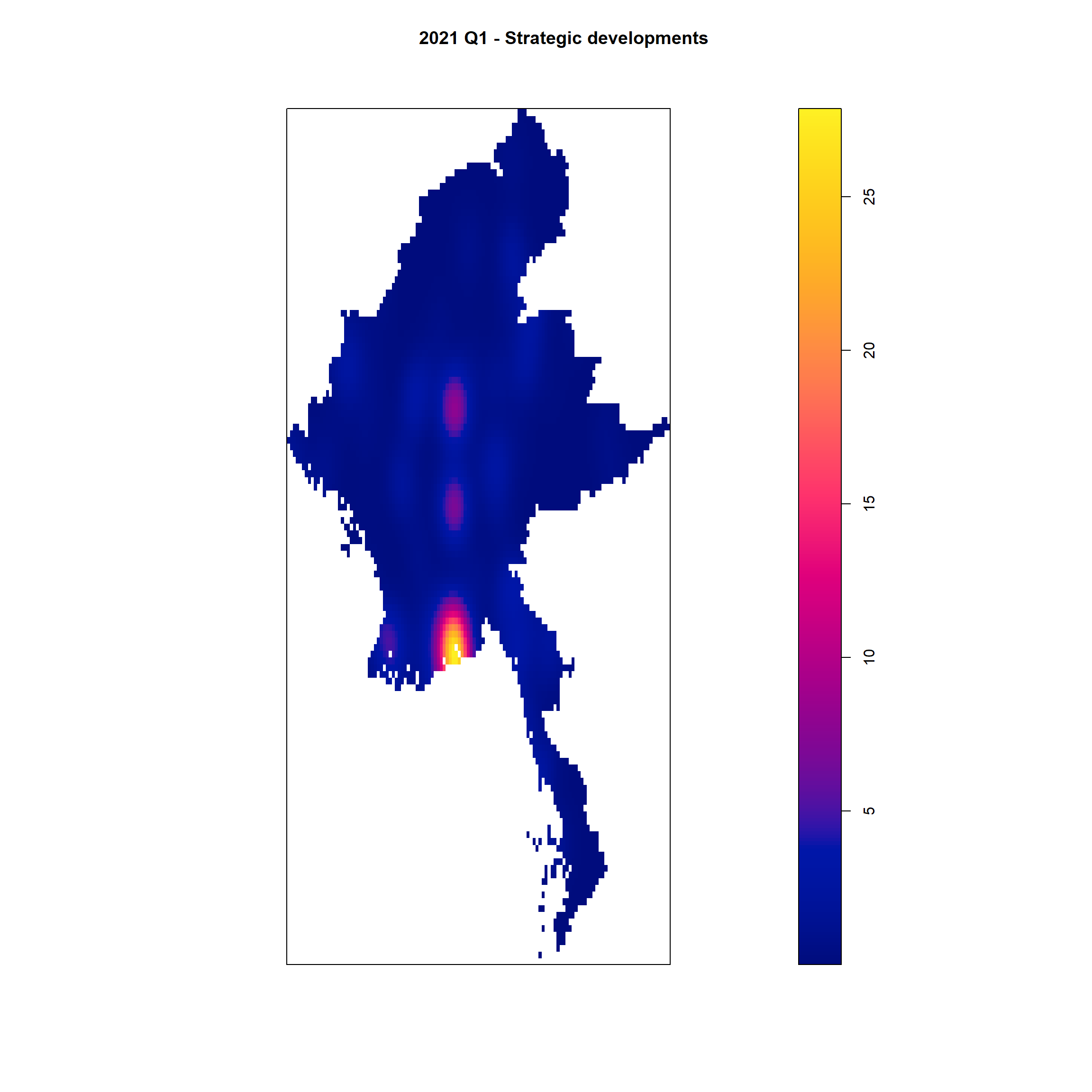
Example <- "Battles"
my_2021_Q1 <- acled_sf  %>%
  filter(event_type == Example & quarter == "2021 Q1")

write_rds(my_2021_Q1, "data/rds/my_2021_Q1_B_quarter_data_regions_sf.rds")

quarter_data <- as_Spatial(my_2021_Q1)
quarter_data_sp <- as(quarter_data, "SpatialPoints")
quarter_data_ppp <- as.ppp(st_coordinates(my_2021_Q1), st_bbox(my_2021_Q1))

quarter_data_ppp_jit <- rjitter(quarter_data_ppp,
                             retry=TRUE,
                             nsim=1,
                             drop=TRUE)
my_2021_Q1_B_quarter_data_regions_ppp = quarter_data_ppp_jit[regions_owin]
quarter_data_regions_ppp.km <- rescale.ppp(my_2021_Q1_B_quarter_data_regions_ppp, 50000, "km")
bw_scott <- bw.scott(quarter_data_regions_ppp.km)
plot(density(quarter_data_regions_ppp.km,
sigma=bw_scott/2,
edge=TRUE,
kernel="gaussian"),
main = "2021 Q1 - Battles")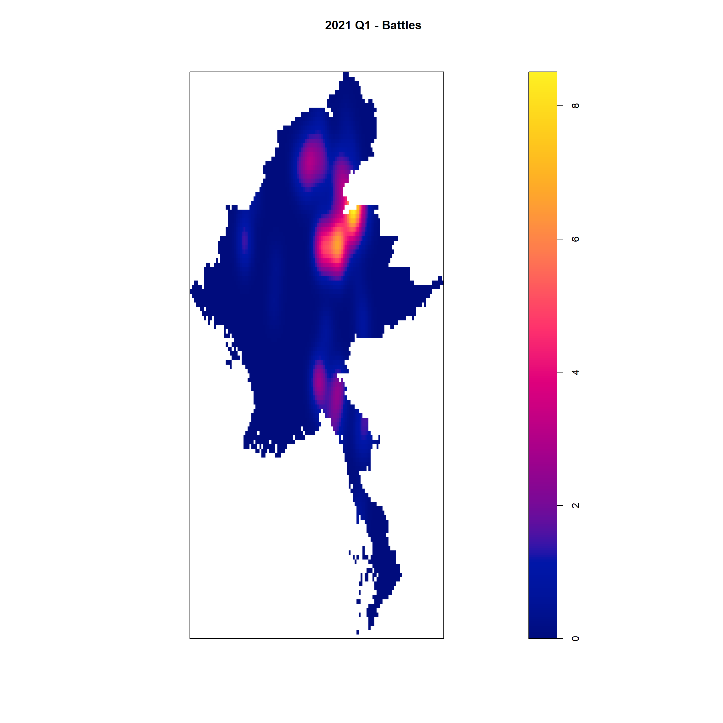
Example <- "Violence against civilians"
my_2021_Q1 <- acled_sf  %>%
  filter(event_type == Example & quarter == "2021 Q1")

write_rds(my_2021_Q1, "data/rds/my_2021_Q1_VAC_quarter_data_regions_sf.rds")

quarter_data <- as_Spatial(my_2021_Q1)
quarter_data_sp <- as(quarter_data, "SpatialPoints")
quarter_data_ppp <- as.ppp(st_coordinates(my_2021_Q1), st_bbox(my_2021_Q1))

quarter_data_ppp_jit <- rjitter(quarter_data_ppp,
                             retry=TRUE,
                             nsim=1,
                             drop=TRUE)
my_2021_Q1_VAC_quarter_data_regions_ppp = quarter_data_ppp_jit[regions_owin]
quarter_data_regions_ppp.km <- rescale.ppp(my_2021_Q1_VAC_quarter_data_regions_ppp, 50000, "km")
bw_scott <- bw.scott(quarter_data_regions_ppp.km)
plot(density(quarter_data_regions_ppp.km,
sigma=bw_scott/2,
edge=TRUE,
kernel="gaussian"),
main = "2021 Q1 -Violence against civilians")
Quarter 2
Example <- "Explosions/Remote violence"
my_2021_Q2 <- acled_sf  %>%
  filter(event_type == Example & quarter == "2021 Q2")

write_rds(my_2021_Q2, "data/rds/my_2021_Q2_ER_quarter_data_regions_sf.rds")

quarter_data <- as_Spatial(my_2021_Q2)
quarter_data_sp <- as(quarter_data, "SpatialPoints")
quarter_data_ppp <- as.ppp(st_coordinates(my_2021_Q2), st_bbox(my_2021_Q2))

quarter_data_ppp_jit <- rjitter(quarter_data_ppp,
                             retry=TRUE,
                             nsim=1,
                             drop=TRUE)
my_2021_Q2_ER_quarter_data_regions_ppp = quarter_data_ppp_jit[regions_owin]
quarter_data_regions_ppp.km <- rescale.ppp(my_2021_Q2_ER_quarter_data_regions_ppp, 50000, "km")
bw_scott <- bw.scott(quarter_data_regions_ppp.km)
plot(density(quarter_data_regions_ppp.km,
sigma=bw_scott/2,
edge=TRUE,
kernel="gaussian"),
main = "2021 Q2 - Explosion/Remote violence")
Example <- "Strategic developments"
my_2021_Q2 <- acled_sf  %>%
  filter(event_type == Example & quarter == "2021 Q2")

write_rds(my_2021_Q2, "data/rds/my_2021_Q2_SD_quarter_data_regions_sf.rds")

quarter_data <- as_Spatial(my_2021_Q2)
quarter_data_sp <- as(quarter_data, "SpatialPoints")
quarter_data_ppp <- as.ppp(st_coordinates(my_2021_Q2), st_bbox(my_2021_Q2))

quarter_data_ppp_jit <- rjitter(quarter_data_ppp,
                             retry=TRUE,
                             nsim=1,
                             drop=TRUE)
my_2021_Q2_SD_quarter_data_regions_ppp = quarter_data_ppp_jit[regions_owin]
quarter_data_regions_ppp.km <- rescale.ppp(my_2021_Q2_SD_quarter_data_regions_ppp, 50000, "km")
bw_scott <- bw.scott(quarter_data_regions_ppp.km)
plot(density(quarter_data_regions_ppp.km,
sigma=bw_scott/2,
edge=TRUE,
kernel="gaussian"),
main = "2021 Q2 - Strategic developments")
Example <- "Battles"
my_2021_Q2 <- acled_sf  %>%
  filter(event_type == Example & quarter == "2021 Q2")

write_rds(my_2021_Q2, "data/rds/my_2021_Q2_B_quarter_data_regions_sf.rds")

quarter_data <- as_Spatial(my_2021_Q2)
quarter_data_sp <- as(quarter_data, "SpatialPoints")
quarter_data_ppp <- as.ppp(st_coordinates(my_2021_Q2), st_bbox(my_2021_Q2))

quarter_data_ppp_jit <- rjitter(quarter_data_ppp,
                             retry=TRUE,
                             nsim=1,
                             drop=TRUE)
my_2021_Q2_B_quarter_data_regions_ppp = quarter_data_ppp_jit[regions_owin]
quarter_data_regions_ppp.km <- rescale.ppp(my_2021_Q2_B_quarter_data_regions_ppp, 50000, "km")
bw_scott <- bw.scott(quarter_data_regions_ppp.km)
plot(density(quarter_data_regions_ppp.km,
sigma=bw_scott/2,
edge=TRUE,
kernel="gaussian"),
main = "2021 Q2 - Battles")
Example <- "Violence against civilians"
my_2021_Q2 <- acled_sf  %>%
  filter(event_type == Example & quarter == "2021 Q2")

write_rds(my_2021_Q2, "data/rds/my_2021_Q2_VAC_quarter_data_regions_sf.rds")

quarter_data <- as_Spatial(my_2021_Q2)
quarter_data_sp <- as(quarter_data, "SpatialPoints")
quarter_data_ppp <- as.ppp(st_coordinates(my_2021_Q2), st_bbox(my_2021_Q2))

quarter_data_ppp_jit <- rjitter(quarter_data_ppp,
                             retry=TRUE,
                             nsim=1,
                             drop=TRUE)
my_2021_Q2_VAC_quarter_data_regions_ppp = quarter_data_ppp_jit[regions_owin]
quarter_data_regions_ppp.km <- rescale.ppp(my_2021_Q2_VAC_quarter_data_regions_ppp, 50000, "km")
bw_scott <- bw.scott(quarter_data_regions_ppp.km)
plot(density(quarter_data_regions_ppp.km,
sigma=bw_scott/2,
edge=TRUE,
kernel="gaussian"),
main = "2021 Q2 - Violence against civilians")
Quarter 3
Example <- "Explosions/Remote violence"
my_2021_Q3 <- acled_sf  %>%
  filter(event_type == Example & quarter == "2021 Q3")

write_rds(my_2021_Q3, "data/rds/my_2021_Q3_ER_quarter_data_regions_sf.rds")

quarter_data <- as_Spatial(my_2021_Q3)
quarter_data_sp <- as(quarter_data, "SpatialPoints")
quarter_data_ppp <- as.ppp(st_coordinates(my_2021_Q3), st_bbox(my_2021_Q3))

quarter_data_ppp_jit <- rjitter(quarter_data_ppp,
                             retry=TRUE,
                             nsim=1,
                             drop=TRUE)
my_2021_Q3_ER_quarter_data_regions_ppp = quarter_data_ppp_jit[regions_owin]
quarter_data_regions_ppp.km <- rescale.ppp(my_2021_Q3_ER_quarter_data_regions_ppp, 50000, "km")
bw_scott <- bw.scott(quarter_data_regions_ppp.km)
plot(density(quarter_data_regions_ppp.km,
sigma=bw_scott/2,
edge=TRUE,
kernel="gaussian"),
main = "2021 Q3 - Explosion/Remote violence")
Example <- "Strategic developments"
my_2021_Q3 <- acled_sf  %>%
  filter(event_type == Example & quarter == "2021 Q3")

write_rds(my_2021_Q3, "data/rds/my_2021_Q3_SD_quarter_data_regions_sf.rds")

quarter_data <- as_Spatial(my_2021_Q3)
quarter_data_sp <- as(quarter_data, "SpatialPoints")
quarter_data_ppp <- as.ppp(st_coordinates(my_2021_Q3), st_bbox(my_2021_Q3))

quarter_data_ppp_jit <- rjitter(quarter_data_ppp,
                             retry=TRUE,
                             nsim=1,
                             drop=TRUE)
my_2021_Q3_SD_quarter_data_regions_ppp = quarter_data_ppp_jit[regions_owin]
quarter_data_regions_ppp.km <- rescale.ppp(my_2021_Q3_SD_quarter_data_regions_ppp, 50000, "km")
bw_scott <- bw.scott(quarter_data_regions_ppp.km)
plot(density(quarter_data_regions_ppp.km,
sigma=bw_scott/2,
edge=TRUE,
kernel="gaussian"),
main = "2021 Q3 - Strategic developments")
Example <- "Battles"
my_2021_Q3 <- acled_sf  %>%
  filter(event_type == Example & quarter == "2021 Q3")

write_rds(my_2021_Q3, "data/rds/my_2021_Q3_B_quarter_data_regions_sf.rds")

quarter_data <- as_Spatial(my_2021_Q3)
quarter_data_sp <- as(quarter_data, "SpatialPoints")
quarter_data_ppp <- as.ppp(st_coordinates(my_2021_Q3), st_bbox(my_2021_Q3))

quarter_data_ppp_jit <- rjitter(quarter_data_ppp,
                             retry=TRUE,
                             nsim=1,
                             drop=TRUE)
my_2021_Q3_B_quarter_data_regions_ppp = quarter_data_ppp_jit[regions_owin]
quarter_data_regions_ppp.km <- rescale.ppp(my_2021_Q3_B_quarter_data_regions_ppp, 50000, "km")
bw_scott <- bw.scott(quarter_data_regions_ppp.km)
plot(density(quarter_data_regions_ppp.km,
sigma=bw_scott/2,
edge=TRUE,
kernel="gaussian"),
main = "2021 Q3 - Battles")
Example <- "Violence against civilians"
my_2021_Q3 <- acled_sf  %>%
  filter(event_type == Example & quarter == "2021 Q3")

write_rds(my_2021_Q3, "data/rds/my_2021_Q3_VAC_quarter_data_regions_sf.rds")

quarter_data <- as_Spatial(my_2021_Q3)
quarter_data_sp <- as(quarter_data, "SpatialPoints")
quarter_data_ppp <- as.ppp(st_coordinates(my_2021_Q3), st_bbox(my_2021_Q3))

quarter_data_ppp_jit <- rjitter(quarter_data_ppp,
                             retry=TRUE,
                             nsim=1,
                             drop=TRUE)
my_2021_Q3_VAC_quarter_data_regions_ppp = quarter_data_ppp_jit[regions_owin]
quarter_data_regions_ppp.km <- rescale.ppp(my_2021_Q3_VAC_quarter_data_regions_ppp, 50000, "km")
bw_scott <- bw.scott(quarter_data_regions_ppp.km)
plot(density(quarter_data_regions_ppp.km,
sigma=bw_scott/2,
edge=TRUE,
kernel="gaussian"),
main = "2021 Q3 - Violence against civilians")
Quarter 4
Example <- "Explosions/Remote violence"
my_2021_Q4 <- acled_sf  %>%
  filter(event_type == Example & quarter == "2021 Q4")

write_rds(my_2021_Q4, "data/rds/my_2021_Q4_ER_quarter_data_regions_sf.rds")

quarter_data <- as_Spatial(my_2021_Q4)
quarter_data_sp <- as(quarter_data, "SpatialPoints")
quarter_data_ppp <- as.ppp(st_coordinates(my_2021_Q4), st_bbox(my_2021_Q4))

quarter_data_ppp_jit <- rjitter(quarter_data_ppp,
                             retry=TRUE,
                             nsim=1,
                             drop=TRUE)
my_2021_Q4_ER_quarter_data_regions_ppp = quarter_data_ppp_jit[regions_owin]
quarter_data_regions_ppp.km <- rescale.ppp(my_2021_Q4_ER_quarter_data_regions_ppp, 50000, "km")
bw_scott <- bw.scott(quarter_data_regions_ppp.km)
plot(density(quarter_data_regions_ppp.km,
sigma=bw_scott/2,
edge=TRUE,
kernel="gaussian"),
main = "2021 Q4 - Explosion/Remote violence")
Example <- "Strategic developments"
my_2021_Q4 <- acled_sf  %>%
  filter(event_type == Example & quarter == "2021 Q4")

write_rds(my_2021_Q4, "data/rds/my_2021_Q4_SD_quarter_data_regions_sf.rds")

quarter_data <- as_Spatial(my_2021_Q4)
quarter_data_sp <- as(quarter_data, "SpatialPoints")
quarter_data_ppp <- as.ppp(st_coordinates(my_2021_Q4), st_bbox(my_2021_Q4))

quarter_data_ppp_jit <- rjitter(quarter_data_ppp,
                             retry=TRUE,
                             nsim=1,
                             drop=TRUE)
my_2021_Q4_SD_quarter_data_regions_ppp = quarter_data_ppp_jit[regions_owin]
quarter_data_regions_ppp.km <- rescale.ppp(my_2021_Q4_SD_quarter_data_regions_ppp, 50000, "km")
bw_scott <- bw.scott(quarter_data_regions_ppp.km)
plot(density(quarter_data_regions_ppp.km,
sigma=bw_scott/2,
edge=TRUE,
kernel="gaussian"),
main = "2021 Q4 - Strategic developments")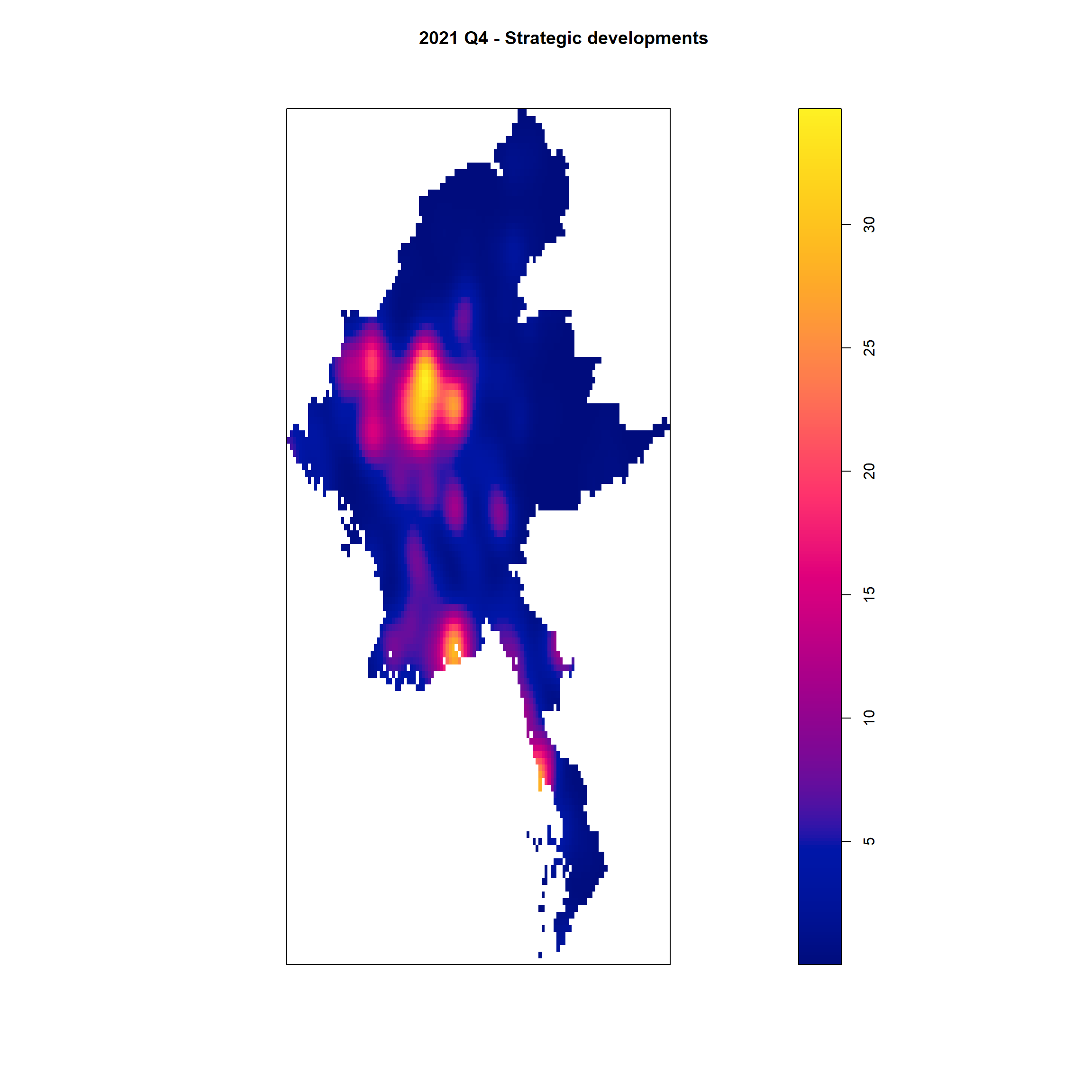
Example <- "Battles"
my_2021_Q4 <- acled_sf  %>%
  filter(event_type == Example & quarter == "2021 Q4")

write_rds(my_2021_Q4, "data/rds/my_2021_Q4_B_quarter_data_regions_sf.rds")

quarter_data <- as_Spatial(my_2021_Q4)
quarter_data_sp <- as(quarter_data, "SpatialPoints")
quarter_data_ppp <- as.ppp(st_coordinates(my_2021_Q4), st_bbox(my_2021_Q4))

quarter_data_ppp_jit <- rjitter(quarter_data_ppp,
                             retry=TRUE,
                             nsim=1,
                             drop=TRUE)
my_2021_Q4_B_quarter_data_regions_ppp = quarter_data_ppp_jit[regions_owin]
quarter_data_regions_ppp.km <- rescale.ppp(my_2021_Q4_B_quarter_data_regions_ppp, 50000, "km")
bw_scott <- bw.scott(quarter_data_regions_ppp.km)
plot(density(quarter_data_regions_ppp.km,
sigma=bw_scott/2,
edge=TRUE,
kernel="gaussian"),
main = "2021 Q4 - Battles")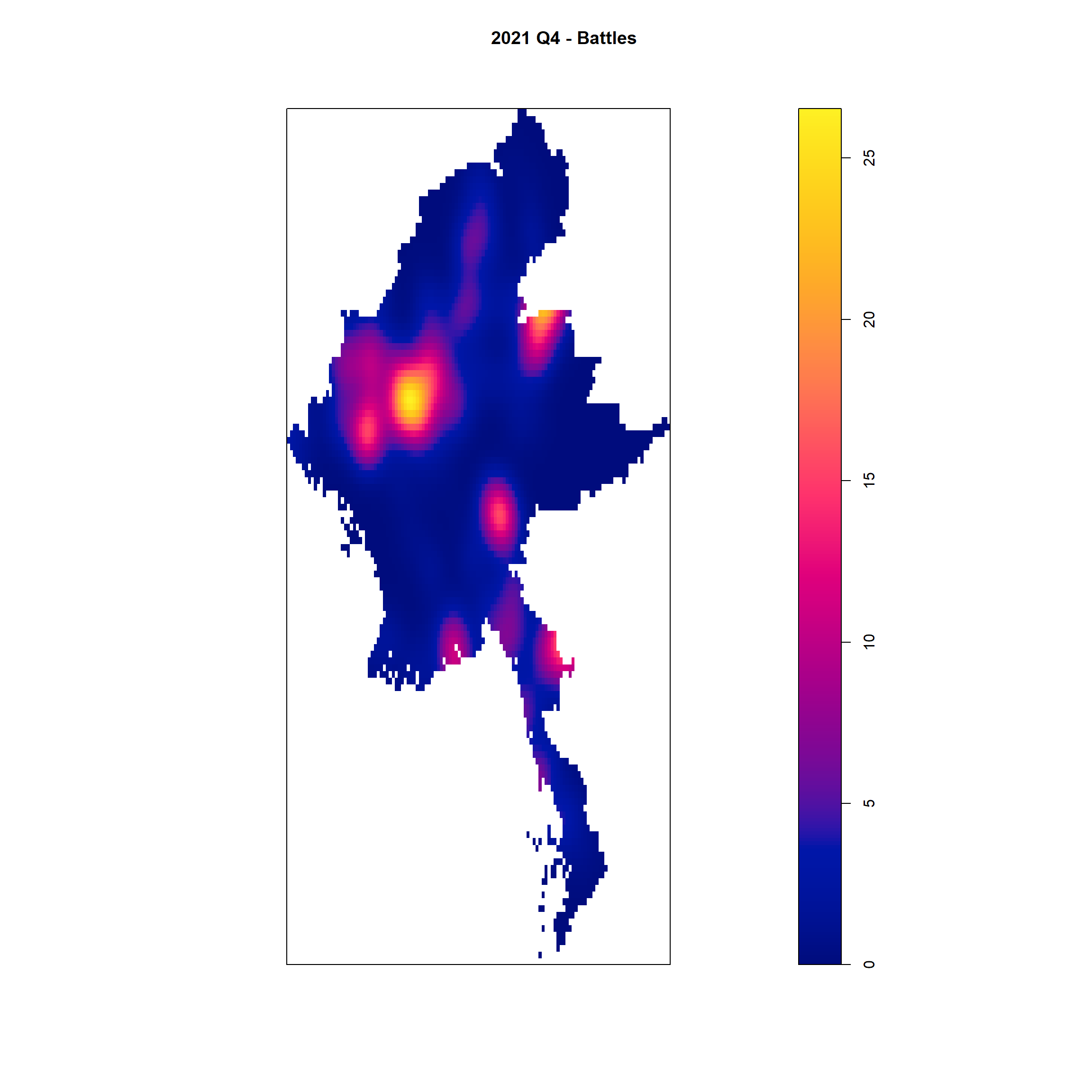
Example <- "Violence against civilians"
my_2021_Q4 <- acled_sf  %>%
  filter(event_type == Example & quarter == "2021 Q4")

write_rds(my_2021_Q4, "data/rds/my_2021_Q4_VAC_quarter_data_regions_sf.rds")

quarter_data <- as_Spatial(my_2021_Q4)
quarter_data_sp <- as(quarter_data, "SpatialPoints")
quarter_data_ppp <- as.ppp(st_coordinates(my_2021_Q4), st_bbox(my_2021_Q4))

quarter_data_ppp_jit <- rjitter(quarter_data_ppp,
                             retry=TRUE,
                             nsim=1,
                             drop=TRUE)
my_2021_Q4_VAC_quarter_data_regions_ppp = quarter_data_ppp_jit[regions_owin]
quarter_data_regions_ppp.km <- rescale.ppp(my_2021_Q4_VAC_quarter_data_regions_ppp, 50000, "km")
bw_scott <- bw.scott(quarter_data_regions_ppp.km)
plot(density(quarter_data_regions_ppp.km,
sigma=bw_scott/2,
edge=TRUE,
kernel="gaussian"),
main = "2021 Q4 - Violence against civilians")
Year 2022
Quarter 1
Example <- "Explosions/Remote violence"
my_2022_Q1 <- acled_sf  %>%
  filter(event_type == Example & quarter == "2022 Q1")

write_rds(my_2022_Q1, "data/rds/my_2022_Q1_ER_quarter_data_regions_sf.rds")

quarter_data <- as_Spatial(my_2022_Q1)
quarter_data_sp <- as(quarter_data, "SpatialPoints")
quarter_data_ppp <- as.ppp(st_coordinates(my_2022_Q1), st_bbox(my_2022_Q1))

quarter_data_ppp_jit <- rjitter(quarter_data_ppp,
                             retry=TRUE,
                             nsim=1,
                             drop=TRUE)
my_2022_Q1_ER_quarter_data_regions_ppp = quarter_data_ppp_jit[regions_owin]
quarter_data_regions_ppp.km <- rescale.ppp(my_2022_Q1_ER_quarter_data_regions_ppp, 50000, "km")
bw_scott <- bw.scott(quarter_data_regions_ppp.km)
plot(density(quarter_data_regions_ppp.km,
sigma=bw_scott/2,
edge=TRUE,
kernel="gaussian"),
main = "2022 Q1 - Explosion/Remote violence")
Example <- "Strategic developments"
my_2022_Q1 <- acled_sf  %>%
  filter(event_type == Example & quarter == "2022 Q1")

write_rds(my_2022_Q1, "data/rds/my_2022_Q1_SD_quarter_data_regions_sf.rds")

quarter_data <- as_Spatial(my_2022_Q1)
quarter_data_sp <- as(quarter_data, "SpatialPoints")
quarter_data_ppp <- as.ppp(st_coordinates(my_2022_Q1), st_bbox(my_2022_Q1))

quarter_data_ppp_jit <- rjitter(quarter_data_ppp,
                             retry=TRUE,
                             nsim=1,
                             drop=TRUE)
my_2022_Q1_SD_quarter_data_regions_ppp = quarter_data_ppp_jit[regions_owin]
quarter_data_regions_ppp.km <- rescale.ppp(my_2022_Q1_SD_quarter_data_regions_ppp, 50000, "km")
bw_scott <- bw.scott(quarter_data_regions_ppp.km)
plot(density(quarter_data_regions_ppp.km,
sigma=bw_scott/2,
edge=TRUE,
kernel="gaussian"),
main = "2022 Q1 - Strategic developments")
Example <- "Battles"
my_2022_Q1 <- acled_sf  %>%
  filter(event_type == Example & quarter == "2022 Q1")

write_rds(my_2022_Q1, "data/rds/my_2022_Q1_B_quarter_data_regions_sf.rds")

quarter_data <- as_Spatial(my_2022_Q1)
quarter_data_sp <- as(quarter_data, "SpatialPoints")
quarter_data_ppp <- as.ppp(st_coordinates(my_2022_Q1), st_bbox(my_2022_Q1))

quarter_data_ppp_jit <- rjitter(quarter_data_ppp,
                             retry=TRUE,
                             nsim=1,
                             drop=TRUE)
my_2022_Q1_B_quarter_data_regions_ppp = quarter_data_ppp_jit[regions_owin]
quarter_data_regions_ppp.km <- rescale.ppp(my_2022_Q1_B_quarter_data_regions_ppp, 50000, "km")
bw_scott <- bw.scott(quarter_data_regions_ppp.km)
plot(density(quarter_data_regions_ppp.km,
sigma=bw_scott/2,
edge=TRUE,
kernel="gaussian"),
main = "2022 Q1 - Battles")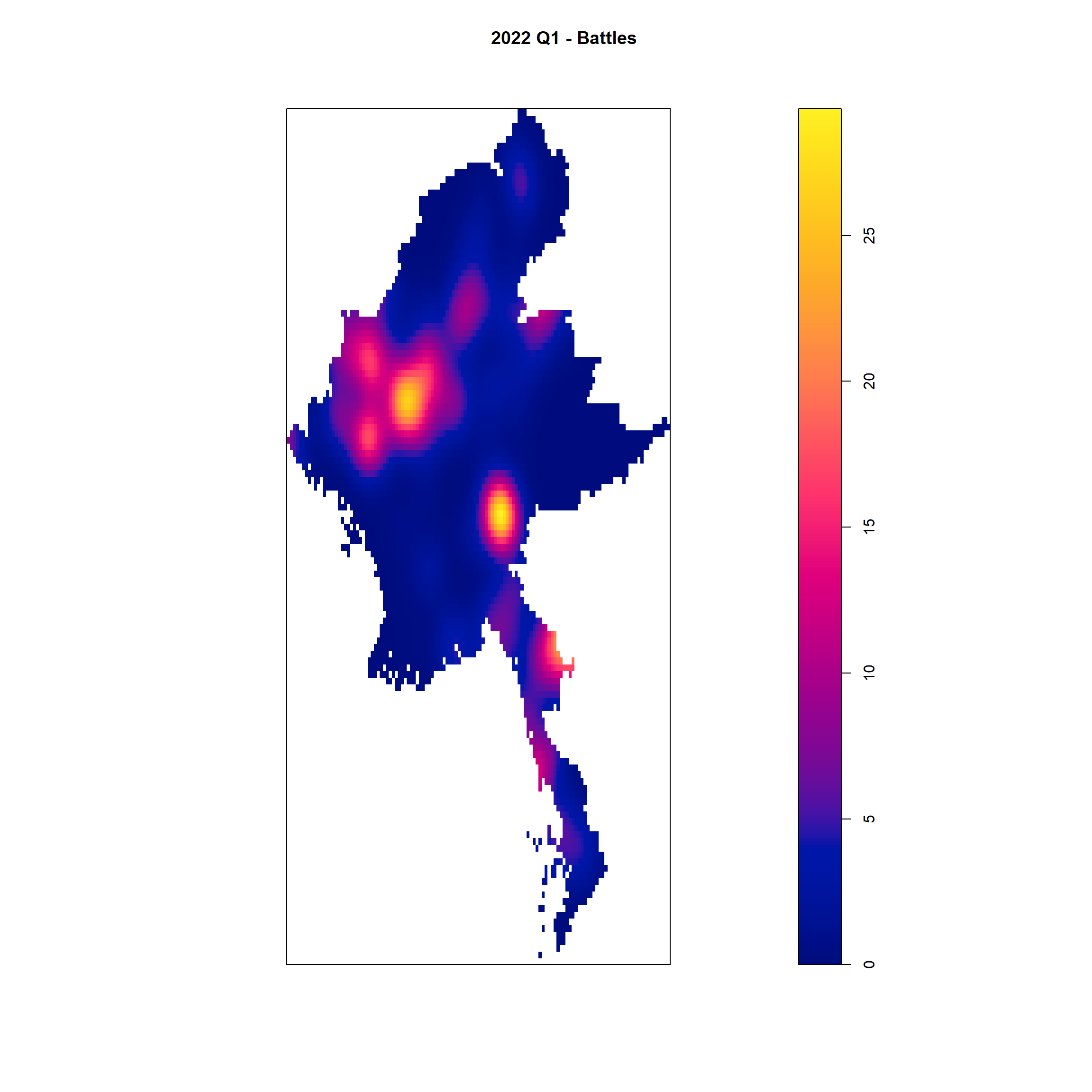
Example <- "Violence against civilians"
my_2022_Q1 <- acled_sf  %>%
  filter(event_type == Example & quarter == "2022 Q1")

write_rds(my_2022_Q1, "data/rds/my_2022_Q1_VAC_quarter_data_regions_sf.rds")

quarter_data <- as_Spatial(my_2022_Q1)
quarter_data_sp <- as(quarter_data, "SpatialPoints")
quarter_data_ppp <- as.ppp(st_coordinates(my_2022_Q1), st_bbox(my_2022_Q1))

quarter_data_ppp_jit <- rjitter(quarter_data_ppp,
                             retry=TRUE,
                             nsim=1,
                             drop=TRUE)
my_2022_Q1_VAC_quarter_data_regions_ppp = quarter_data_ppp_jit[regions_owin]
quarter_data_regions_ppp.km <- rescale.ppp(my_2022_Q1_VAC_quarter_data_regions_ppp, 50000, "km")
bw_scott <- bw.scott(quarter_data_regions_ppp.km)
plot(density(quarter_data_regions_ppp.km,
sigma=bw_scott/2,
edge=TRUE,
kernel="gaussian"),
main = "2022 Q1 -Violence against civilians")
Quarter 2
Example <- "Explosions/Remote violence"
my_2022_Q2 <- acled_sf  %>%
  filter(event_type == Example & quarter == "2022 Q2")

write_rds(my_2022_Q2, "data/rds/my_2022_Q2_ER_quarter_data_regions_sf.rds")

quarter_data <- as_Spatial(my_2022_Q2)
quarter_data_sp <- as(quarter_data, "SpatialPoints")
quarter_data_ppp <- as.ppp(st_coordinates(my_2022_Q2), st_bbox(my_2022_Q2))

quarter_data_ppp_jit <- rjitter(quarter_data_ppp,
                             retry=TRUE,
                             nsim=1,
                             drop=TRUE)
my_2022_Q2_ER_quarter_data_regions_ppp = quarter_data_ppp_jit[regions_owin]
quarter_data_regions_ppp.km <- rescale.ppp(my_2022_Q2_ER_quarter_data_regions_ppp, 50000, "km")
bw_scott <- bw.scott(quarter_data_regions_ppp.km)
plot(density(quarter_data_regions_ppp.km,
sigma=bw_scott/2,
edge=TRUE,
kernel="gaussian"),
main = "2022 Q2 - Explosion/Remote violence")
Example <- "Strategic developments"
my_2022_Q2 <- acled_sf  %>%
  filter(event_type == Example & quarter == "2022 Q2")

write_rds(my_2022_Q2, "data/rds/my_2022_Q2_SD_quarter_data_regions_sf.rds")

quarter_data <- as_Spatial(my_2022_Q2)
quarter_data_sp <- as(quarter_data, "SpatialPoints")
quarter_data_ppp <- as.ppp(st_coordinates(my_2022_Q2), st_bbox(my_2022_Q2))

quarter_data_ppp_jit <- rjitter(quarter_data_ppp,
                             retry=TRUE,
                             nsim=1,
                             drop=TRUE)
my_2022_Q2_SD_quarter_data_regions_ppp = quarter_data_ppp_jit[regions_owin]
quarter_data_regions_ppp.km <- rescale.ppp(my_2022_Q2_SD_quarter_data_regions_ppp, 50000, "km")
bw_scott <- bw.scott(quarter_data_regions_ppp.km)
plot(density(quarter_data_regions_ppp.km,
sigma=bw_scott/2,
edge=TRUE,
kernel="gaussian"),
main = "2022 Q2 - Strategic developments")
Example <- "Battles"
my_2022_Q2 <- acled_sf  %>%
  filter(event_type == Example & quarter == "2022 Q2")

write_rds(my_2022_Q2, "data/rds/my_2022_Q2_B_quarter_data_regions_sf.rds")

quarter_data <- as_Spatial(my_2022_Q2)
quarter_data_sp <- as(quarter_data, "SpatialPoints")
quarter_data_ppp <- as.ppp(st_coordinates(my_2022_Q2), st_bbox(my_2022_Q2))

quarter_data_ppp_jit <- rjitter(quarter_data_ppp,
                             retry=TRUE,
                             nsim=1,
                             drop=TRUE)
my_2022_Q2_B_quarter_data_regions_ppp = quarter_data_ppp_jit[regions_owin]
quarter_data_regions_ppp.km <- rescale.ppp(my_2022_Q2_B_quarter_data_regions_ppp, 50000, "km")
bw_scott <- bw.scott(quarter_data_regions_ppp.km)
plot(density(quarter_data_regions_ppp.km,
sigma=bw_scott/2,
edge=TRUE,
kernel="gaussian"),
main = "2022 Q2 - Battles")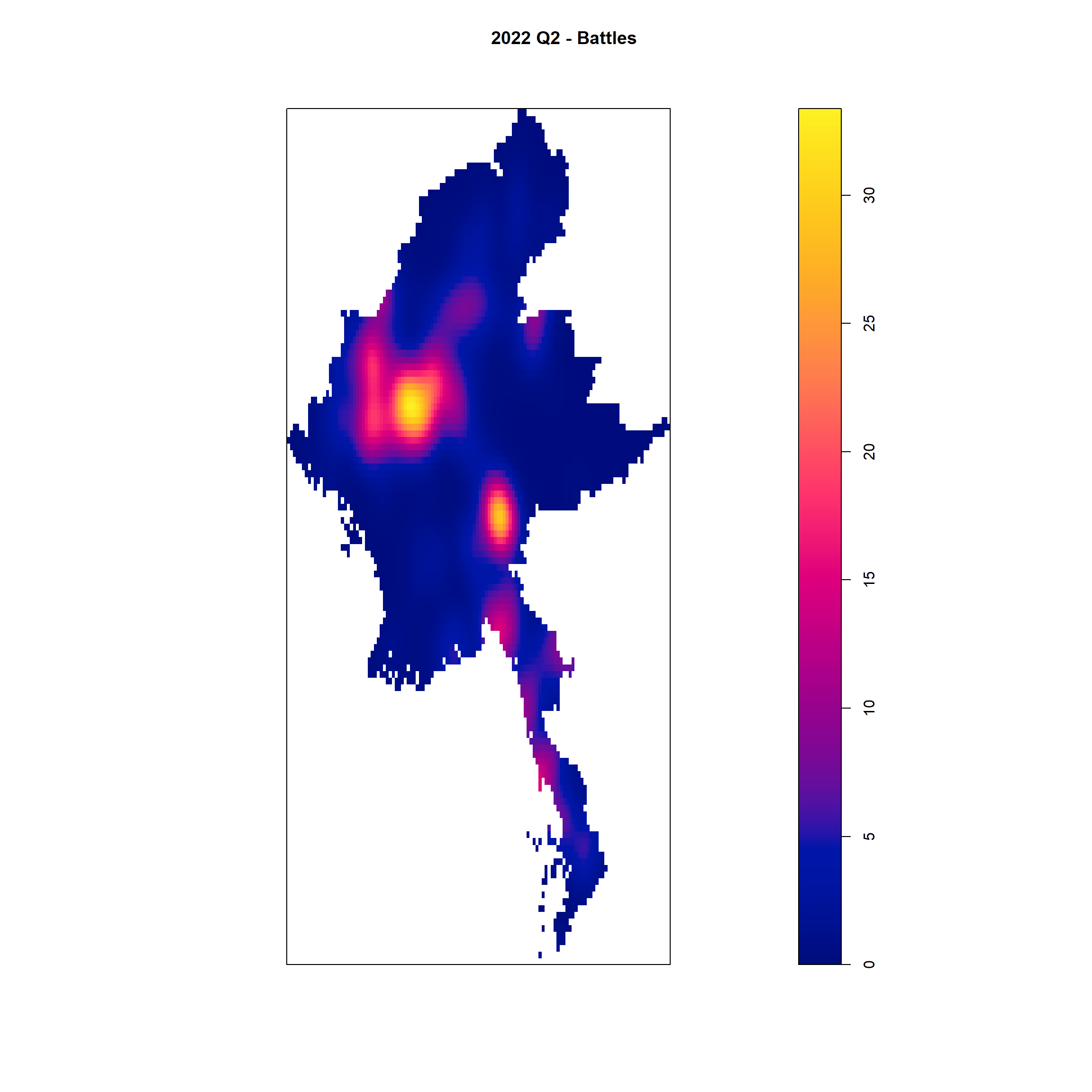
Example <- "Violence against civilians"
my_2022_Q2 <- acled_sf  %>%
  filter(event_type == Example & quarter == "2022 Q2")

write_rds(my_2022_Q2, "data/rds/my_2022_Q2_VAC_quarter_data_regions_sf.rds")

quarter_data <- as_Spatial(my_2022_Q2)
quarter_data_sp <- as(quarter_data, "SpatialPoints")
quarter_data_ppp <- as.ppp(st_coordinates(my_2022_Q2), st_bbox(my_2022_Q2))

quarter_data_ppp_jit <- rjitter(quarter_data_ppp,
                             retry=TRUE,
                             nsim=1,
                             drop=TRUE)
my_2022_Q2_VAC_quarter_data_regions_ppp = quarter_data_ppp_jit[regions_owin]
quarter_data_regions_ppp.km <- rescale.ppp(my_2022_Q2_VAC_quarter_data_regions_ppp, 50000, "km")
bw_scott <- bw.scott(quarter_data_regions_ppp.km)
plot(density(quarter_data_regions_ppp.km,
sigma=bw_scott/2,
edge=TRUE,
kernel="gaussian"),
main = "2022 Q2 - Violence against civilians")
Quarter 3
Example <- "Explosions/Remote violence"
my_2022_Q3 <- acled_sf  %>%
  filter(event_type == Example & quarter == "2022 Q3")

write_rds(my_2022_Q3, "data/rds/my_2022_Q3_ER_quarter_data_regions_sf.rds")

quarter_data <- as_Spatial(my_2022_Q3)
quarter_data_sp <- as(quarter_data, "SpatialPoints")
quarter_data_ppp <- as.ppp(st_coordinates(my_2022_Q3), st_bbox(my_2022_Q3))

quarter_data_ppp_jit <- rjitter(quarter_data_ppp,
                             retry=TRUE,
                             nsim=1,
                             drop=TRUE)
my_2022_Q3_ER_quarter_data_regions_ppp = quarter_data_ppp_jit[regions_owin]
quarter_data_regions_ppp.km <- rescale.ppp(my_2022_Q3_ER_quarter_data_regions_ppp, 50000, "km")
bw_scott <- bw.scott(quarter_data_regions_ppp.km)
plot(density(quarter_data_regions_ppp.km,
sigma=bw_scott/2,
edge=TRUE,
kernel="gaussian"),
main = "2022 Q3 - Explosion/Remote violence")
Example <- "Strategic developments"
my_2022_Q3 <- acled_sf  %>%
  filter(event_type == Example & quarter == "2022 Q3")

write_rds(my_2022_Q3, "data/rds/my_2022_Q3_SD_quarter_data_regions_sf.rds")

quarter_data <- as_Spatial(my_2022_Q3)
quarter_data_sp <- as(quarter_data, "SpatialPoints")
quarter_data_ppp <- as.ppp(st_coordinates(my_2022_Q3), st_bbox(my_2022_Q3))

quarter_data_ppp_jit <- rjitter(quarter_data_ppp,
                             retry=TRUE,
                             nsim=1,
                             drop=TRUE)
my_2022_Q3_SD_quarter_data_regions_ppp = quarter_data_ppp_jit[regions_owin]
quarter_data_regions_ppp.km <- rescale.ppp(my_2022_Q3_SD_quarter_data_regions_ppp, 50000, "km")
bw_scott <- bw.scott(quarter_data_regions_ppp.km)
plot(density(quarter_data_regions_ppp.km,
sigma=bw_scott/2,
edge=TRUE,
kernel="gaussian"),
main = "2022 Q3 - Strategic developments")
Example <- "Battles"
my_2022_Q3 <- acled_sf  %>%
  filter(event_type == Example & quarter == "2022 Q3")

write_rds(my_2022_Q3, "data/rds/my_2022_Q3_B_quarter_data_regions_sf.rds")

quarter_data <- as_Spatial(my_2022_Q3)
quarter_data_sp <- as(quarter_data, "SpatialPoints")
quarter_data_ppp <- as.ppp(st_coordinates(my_2022_Q3), st_bbox(my_2022_Q3))

quarter_data_ppp_jit <- rjitter(quarter_data_ppp,
                             retry=TRUE,
                             nsim=1,
                             drop=TRUE)
my_2022_Q3_B_quarter_data_regions_ppp = quarter_data_ppp_jit[regions_owin]
quarter_data_regions_ppp.km <- rescale.ppp(my_2022_Q3_B_quarter_data_regions_ppp, 50000, "km")
bw_scott <- bw.scott(quarter_data_regions_ppp.km)
plot(density(quarter_data_regions_ppp.km,
sigma=bw_scott/2,
edge=TRUE,
kernel="gaussian"),
main = "2022 Q3 - Battles")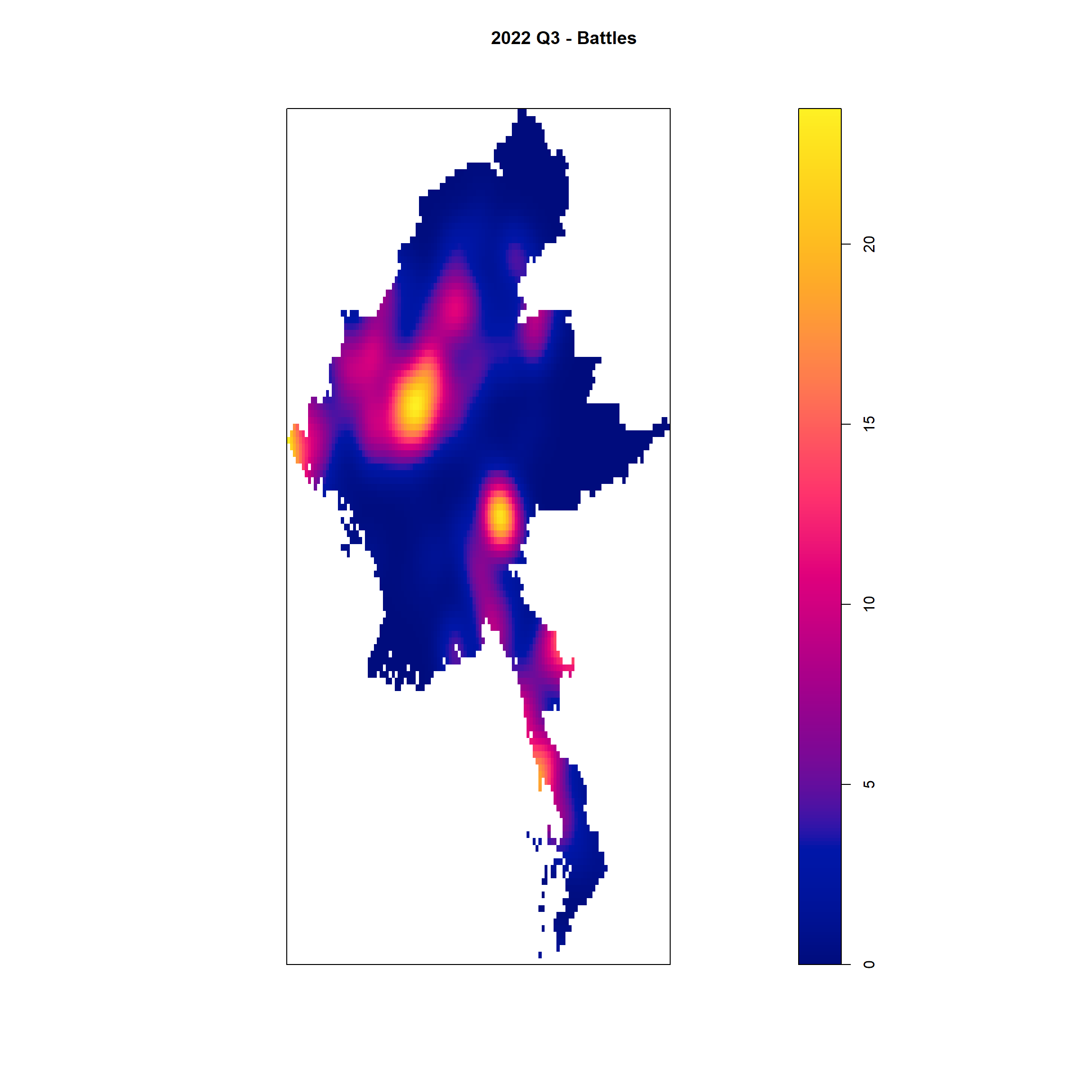
Example <- "Violence against civilians"
my_2022_Q3 <- acled_sf  %>%
  filter(event_type == Example & quarter == "2022 Q3")

write_rds(my_2022_Q3, "data/rds/my_2022_Q3_VAC_quarter_data_regions_sf.rds")

quarter_data <- as_Spatial(my_2022_Q3)
quarter_data_sp <- as(quarter_data, "SpatialPoints")
quarter_data_ppp <- as.ppp(st_coordinates(my_2022_Q3), st_bbox(my_2022_Q3))

quarter_data_ppp_jit <- rjitter(quarter_data_ppp,
                             retry=TRUE,
                             nsim=1,
                             drop=TRUE)
my_2022_Q3_VAC_quarter_data_regions_ppp = quarter_data_ppp_jit[regions_owin]
quarter_data_regions_ppp.km <- rescale.ppp(my_2022_Q3_VAC_quarter_data_regions_ppp, 50000, "km")
bw_scott <- bw.scott(quarter_data_regions_ppp.km)
plot(density(quarter_data_regions_ppp.km,
sigma=bw_scott/2,
edge=TRUE,
kernel="gaussian"),
main = "2022 Q3 - Violence against civilians")
Quarter 4
Example <- "Explosions/Remote violence"
my_2022_Q4 <- acled_sf  %>%
  filter(event_type == Example & quarter == "2022 Q4")

write_rds(my_2022_Q4, "data/rds/my_2022_Q4_ER_quarter_data_regions_sf.rds")

quarter_data <- as_Spatial(my_2022_Q4)
quarter_data_sp <- as(quarter_data, "SpatialPoints")
quarter_data_ppp <- as.ppp(st_coordinates(my_2022_Q4), st_bbox(my_2022_Q4))

quarter_data_ppp_jit <- rjitter(quarter_data_ppp,
                             retry=TRUE,
                             nsim=1,
                             drop=TRUE)
my_2022_Q4_ER_quarter_data_regions_ppp = quarter_data_ppp_jit[regions_owin]
quarter_data_regions_ppp.km <- rescale.ppp(my_2022_Q4_ER_quarter_data_regions_ppp, 50000, "km")
bw_scott <- bw.scott(quarter_data_regions_ppp.km)
plot(density(quarter_data_regions_ppp.km,
sigma=bw_scott/2,
edge=TRUE,
kernel="gaussian"),
main = "2022 Q4 - Explosion/Remote violence")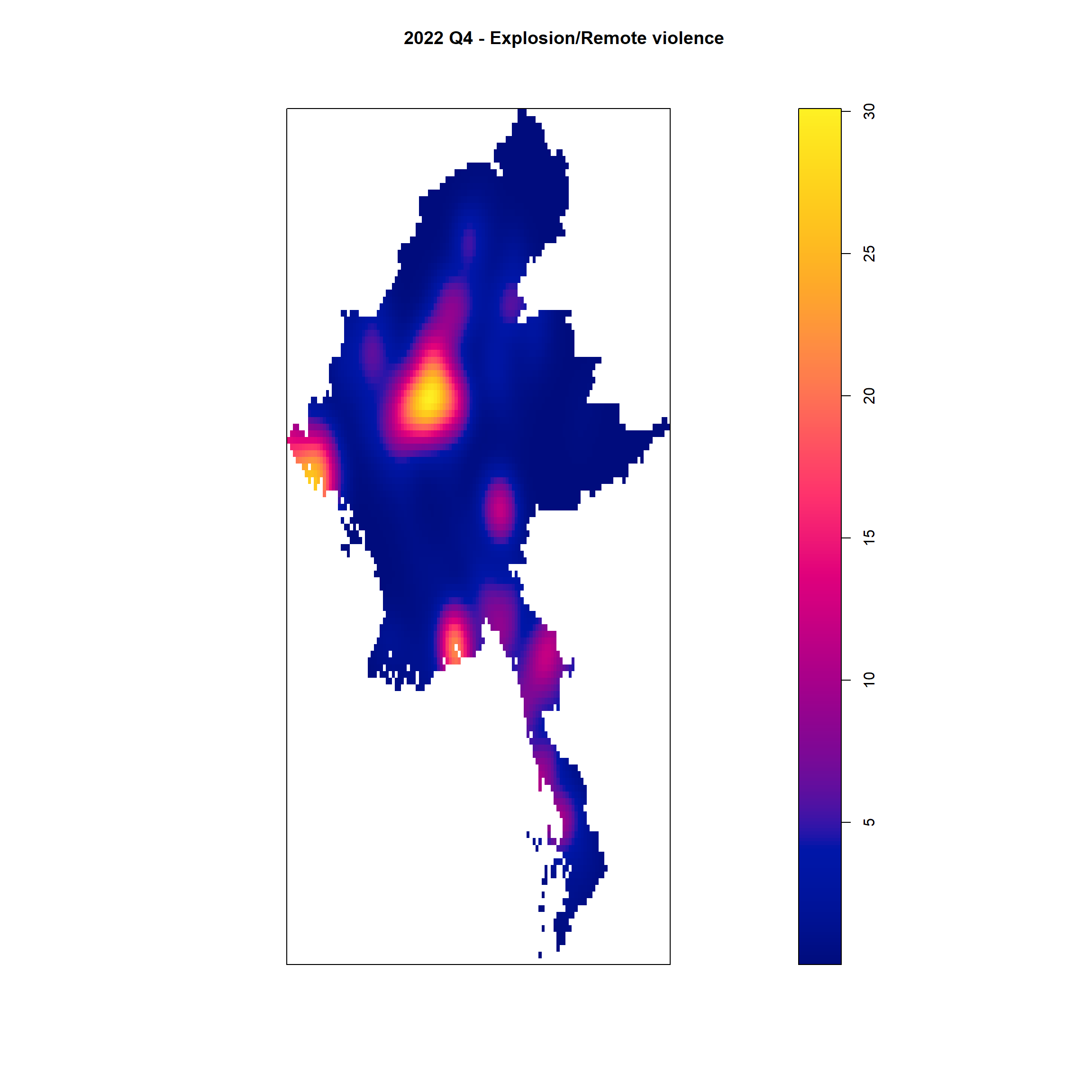
Example <- "Strategic developments"
my_2022_Q4 <- acled_sf  %>%
  filter(event_type == Example & quarter == "2022 Q4")

write_rds(my_2022_Q4, "data/rds/my_2022_Q4_SD_quarter_data_regions_sf.rds")

quarter_data <- as_Spatial(my_2022_Q4)
quarter_data_sp <- as(quarter_data, "SpatialPoints")
quarter_data_ppp <- as.ppp(st_coordinates(my_2022_Q4), st_bbox(my_2022_Q4))

quarter_data_ppp_jit <- rjitter(quarter_data_ppp,
                             retry=TRUE,
                             nsim=1,
                             drop=TRUE)
my_2022_Q4_SD_quarter_data_regions_ppp = quarter_data_ppp_jit[regions_owin]
quarter_data_regions_ppp.km <- rescale.ppp(my_2022_Q4_SD_quarter_data_regions_ppp, 50000, "km")
bw_scott <- bw.scott(quarter_data_regions_ppp.km)
plot(density(quarter_data_regions_ppp.km,
sigma=bw_scott/2,
edge=TRUE,
kernel="gaussian"),
main = "2022 Q4 - Strategic developments")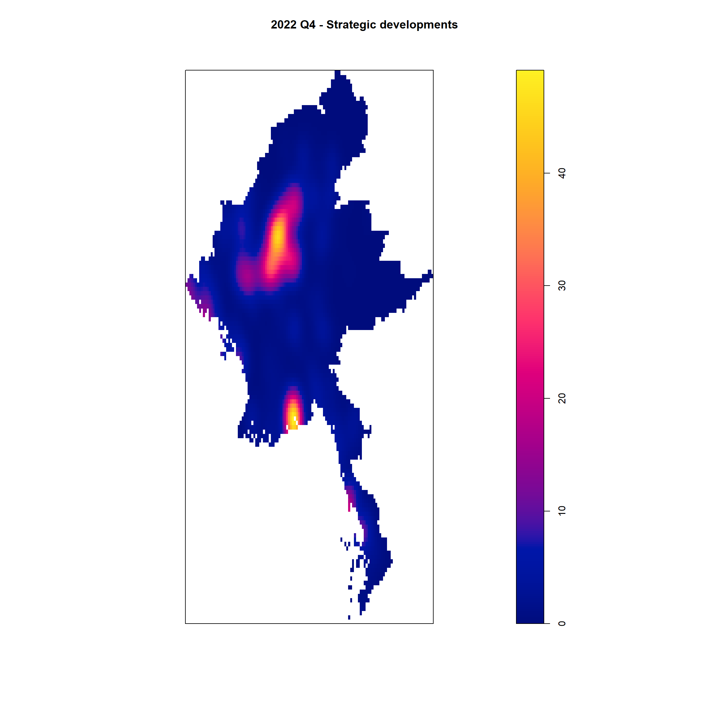
Example <- "Battles"
my_2022_Q4 <- acled_sf  %>%
  filter(event_type == Example & quarter == "2022 Q4")

write_rds(my_2022_Q4, "data/rds/my_2022_Q4_B_quarter_data_regions_sf.rds")

quarter_data <- as_Spatial(my_2022_Q4)
quarter_data_sp <- as(quarter_data, "SpatialPoints")
quarter_data_ppp <- as.ppp(st_coordinates(my_2022_Q4), st_bbox(my_2022_Q4))

quarter_data_ppp_jit <- rjitter(quarter_data_ppp,
                             retry=TRUE,
                             nsim=1,
                             drop=TRUE)
my_2022_Q4_B_quarter_data_regions_ppp = quarter_data_ppp_jit[regions_owin]
quarter_data_regions_ppp.km <- rescale.ppp(my_2022_Q4_B_quarter_data_regions_ppp, 50000, "km")
bw_scott <- bw.scott(quarter_data_regions_ppp.km)
plot(density(quarter_data_regions_ppp.km,
sigma=bw_scott/2,
edge=TRUE,
kernel="gaussian"),
main = "2022 Q4 - Battles")
Example <- "Violence against civilians"
my_2022_Q4 <- acled_sf  %>%
  filter(event_type == Example & quarter == "2022 Q4")

write_rds(my_2022_Q4, "data/rds/my_2022_Q4_VAC_quarter_data_regions_sf.rds")

quarter_data <- as_Spatial(my_2022_Q4)
quarter_data_sp <- as(quarter_data, "SpatialPoints")
quarter_data_ppp <- as.ppp(st_coordinates(my_2022_Q4), st_bbox(my_2022_Q4))

quarter_data_ppp_jit <- rjitter(quarter_data_ppp,
                             retry=TRUE,
                             nsim=1,
                             drop=TRUE)
my_2022_Q4_VAC_quarter_data_regions_ppp = quarter_data_ppp_jit[regions_owin]
quarter_data_regions_ppp.km <- rescale.ppp(my_2022_Q4_VAC_quarter_data_regions_ppp, 50000, "km")
bw_scott <- bw.scott(quarter_data_regions_ppp.km)
plot(density(quarter_data_regions_ppp.km,
sigma=bw_scott/2,
edge=TRUE,
kernel="gaussian"),
main = "2022 Q4 - Violence against civilians")
Year 2023
Quarter 1
Example <- "Explosions/Remote violence"
my_2023_Q1 <- acled_sf  %>%
  filter(event_type == Example & quarter == "2023 Q1")

write_rds(my_2023_Q1, "data/rds/my_2023_Q1_ER_quarter_data_regions_sf.rds")

quarter_data <- as_Spatial(my_2023_Q1)
quarter_data_sp <- as(quarter_data, "SpatialPoints")
quarter_data_ppp <- as.ppp(st_coordinates(my_2023_Q1), st_bbox(my_2023_Q1))

quarter_data_ppp_jit <- rjitter(quarter_data_ppp,
                             retry=TRUE,
                             nsim=1,
                             drop=TRUE)
my_2023_Q1_ER_quarter_data_regions_ppp = quarter_data_ppp_jit[regions_owin]
quarter_data_regions_ppp.km <- rescale.ppp(my_2023_Q1_ER_quarter_data_regions_ppp, 50000, "km")
bw_scott <- bw.scott(quarter_data_regions_ppp.km)
plot(density(quarter_data_regions_ppp.km,
sigma=bw_scott/2,
edge=TRUE,
kernel="gaussian"),
main = "2023 Q1 - Explosion/Remote violence")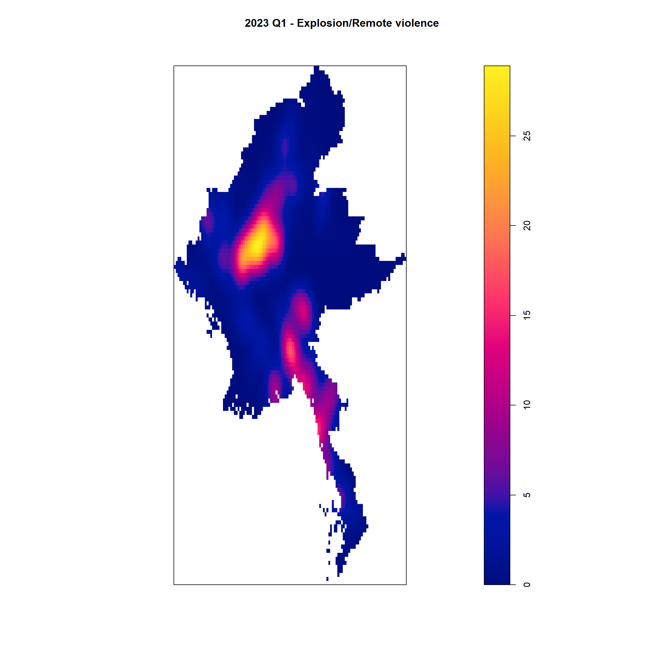
Example <- "Strategic developments"
my_2023_Q1 <- acled_sf  %>%
  filter(event_type == Example & quarter == "2023 Q1")

write_rds(my_2023_Q1, "data/rds/my_2023_Q1_SD_quarter_data_regions_sf.rds")

quarter_data <- as_Spatial(my_2023_Q1)
quarter_data_sp <- as(quarter_data, "SpatialPoints")
quarter_data_ppp <- as.ppp(st_coordinates(my_2023_Q1), st_bbox(my_2023_Q1))

quarter_data_ppp_jit <- rjitter(quarter_data_ppp,
                             retry=TRUE,
                             nsim=1,
                             drop=TRUE)
my_2023_Q1_SD_quarter_data_regions_ppp = quarter_data_ppp_jit[regions_owin]
quarter_data_regions_ppp.km <- rescale.ppp(my_2023_Q1_SD_quarter_data_regions_ppp, 50000, "km")
bw_scott <- bw.scott(quarter_data_regions_ppp.km)
plot(density(quarter_data_regions_ppp.km,
sigma=bw_scott/2,
edge=TRUE,
kernel="gaussian"),
main = "2023 Q1 - Strategic developments")
Example <- "Battles"
my_2023_Q1 <- acled_sf  %>%
  filter(event_type == Example & quarter == "2023 Q1")

write_rds(my_2023_Q1, "data/rds/my_2023_Q1_B_quarter_data_regions_sf.rds")

quarter_data <- as_Spatial(my_2023_Q1)
quarter_data_sp <- as(quarter_data, "SpatialPoints")
quarter_data_ppp <- as.ppp(st_coordinates(my_2023_Q1), st_bbox(my_2023_Q1))

quarter_data_ppp_jit <- rjitter(quarter_data_ppp,
                             retry=TRUE,
                             nsim=1,
                             drop=TRUE)
my_2023_Q1_B_quarter_data_regions_ppp = quarter_data_ppp_jit[regions_owin]
quarter_data_regions_ppp.km <- rescale.ppp(my_2023_Q1_B_quarter_data_regions_ppp, 50000, "km")
bw_scott <- bw.scott(quarter_data_regions_ppp.km)
plot(density(quarter_data_regions_ppp.km,
sigma=bw_scott/2,
edge=TRUE,
kernel="gaussian"),
main = "2023 Q1 - Battles")
Example <- "Violence against civilians"
my_2023_Q1 <- acled_sf  %>%
  filter(event_type == Example & quarter == "2023 Q1")

write_rds(my_2023_Q1, "data/rds/my_2023_Q1_VAC_quarter_data_regions_sf.rds")

quarter_data <- as_Spatial(my_2023_Q1)
quarter_data_sp <- as(quarter_data, "SpatialPoints")
quarter_data_ppp <- as.ppp(st_coordinates(my_2023_Q1), st_bbox(my_2023_Q1))

quarter_data_ppp_jit <- rjitter(quarter_data_ppp,
                             retry=TRUE,
                             nsim=1,
                             drop=TRUE)
my_2023_Q1_VAC_quarter_data_regions_ppp = quarter_data_ppp_jit[regions_owin]
quarter_data_regions_ppp.km <- rescale.ppp(my_2023_Q1_VAC_quarter_data_regions_ppp, 50000, "km")
bw_scott <- bw.scott(quarter_data_regions_ppp.km)
plot(density(quarter_data_regions_ppp.km,
sigma=bw_scott/2,
edge=TRUE,
kernel="gaussian"),
main = "2023 Q1 -Violence against civilians")
Quarter 2
Example <- "Explosions/Remote violence"
my_2023_Q2 <- acled_sf  %>%
  filter(event_type == Example & quarter == "2023 Q2")

write_rds(my_2023_Q2, "data/rds/my_2023_Q2_ER_quarter_data_regions_sf.rds")

quarter_data <- as_Spatial(my_2023_Q2)
quarter_data_sp <- as(quarter_data, "SpatialPoints")
quarter_data_ppp <- as.ppp(st_coordinates(my_2023_Q2), st_bbox(my_2023_Q2))

quarter_data_ppp_jit <- rjitter(quarter_data_ppp,
                             retry=TRUE,
                             nsim=1,
                             drop=TRUE)
my_2023_Q2_ER_quarter_data_regions_ppp = quarter_data_ppp_jit[regions_owin]
quarter_data_regions_ppp.km <- rescale.ppp(my_2023_Q2_ER_quarter_data_regions_ppp, 50000, "km")
bw_scott <- bw.scott(quarter_data_regions_ppp.km)
plot(density(quarter_data_regions_ppp.km,
sigma=bw_scott/2,
edge=TRUE,
kernel="gaussian"),
main = "2023 Q2 - Explosion/Remote violence")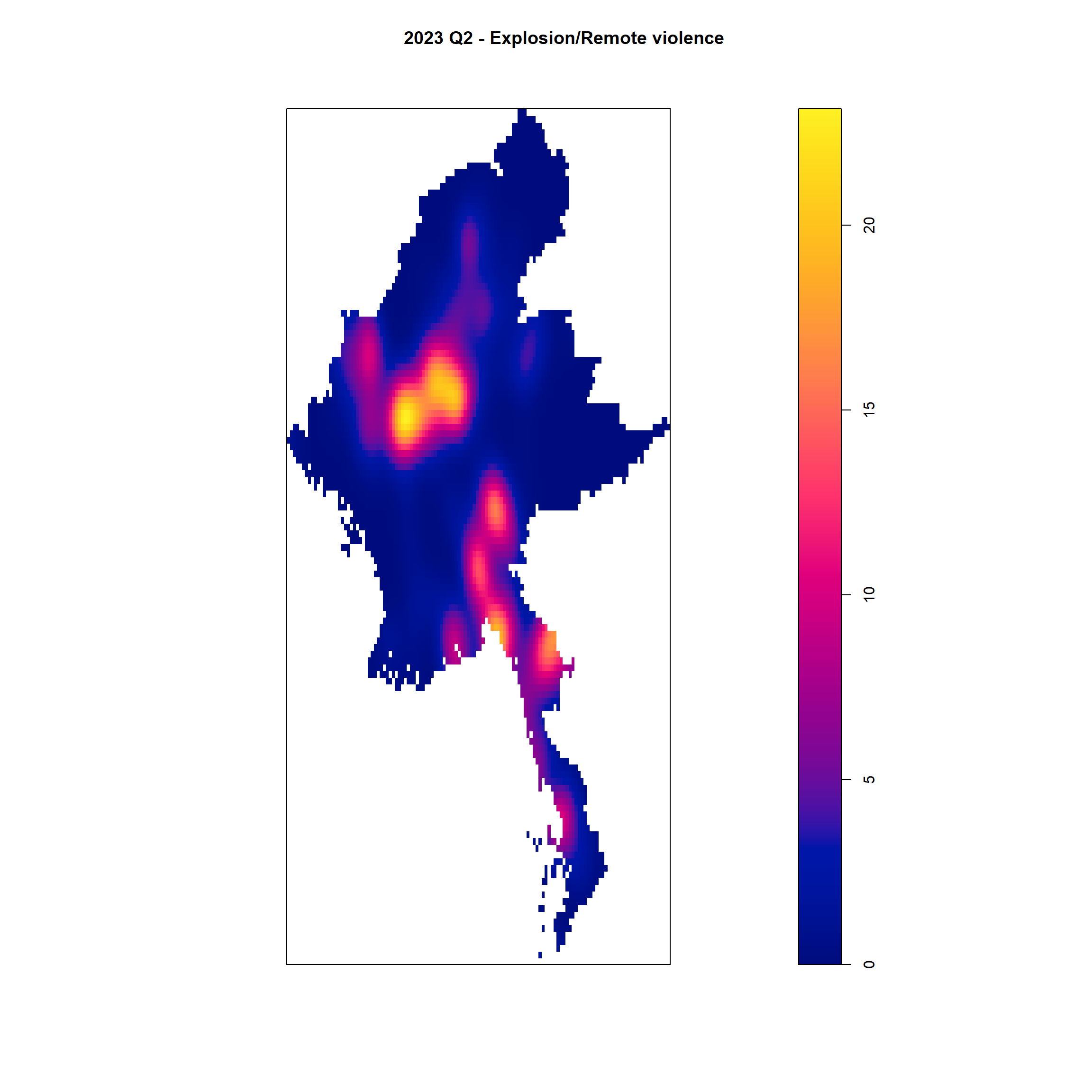
Example <- "Strategic developments"
my_2023_Q2 <- acled_sf  %>%
  filter(event_type == Example & quarter == "2023 Q2")

write_rds(my_2023_Q2, "data/rds/my_2023_Q2_SD_quarter_data_regions_sf.rds")

quarter_data <- as_Spatial(my_2023_Q2)
quarter_data_sp <- as(quarter_data, "SpatialPoints")
quarter_data_ppp <- as.ppp(st_coordinates(my_2023_Q2), st_bbox(my_2023_Q2))

quarter_data_ppp_jit <- rjitter(quarter_data_ppp,
                             retry=TRUE,
                             nsim=1,
                             drop=TRUE)
my_2023_Q2_SD_quarter_data_regions_ppp = quarter_data_ppp_jit[regions_owin]
quarter_data_regions_ppp.km <- rescale.ppp(my_2023_Q2_SD_quarter_data_regions_ppp, 50000, "km")
bw_scott <- bw.scott(quarter_data_regions_ppp.km)
plot(density(quarter_data_regions_ppp.km,
sigma=bw_scott/2,
edge=TRUE,
kernel="gaussian"),
main = "2023 Q2 - Strategic developments")
Example <- "Battles"
my_2023_Q2 <- acled_sf  %>%
  filter(event_type == Example & quarter == "2023 Q2")

write_rds(my_2023_Q2, "data/rds/my_2023_Q2_B_quarter_data_regions_sf.rds")

quarter_data <- as_Spatial(my_2023_Q2)
quarter_data_sp <- as(quarter_data, "SpatialPoints")
quarter_data_ppp <- as.ppp(st_coordinates(my_2023_Q2), st_bbox(my_2023_Q2))

quarter_data_ppp_jit <- rjitter(quarter_data_ppp,
                             retry=TRUE,
                             nsim=1,
                             drop=TRUE)
my_2023_Q2_B_quarter_data_regions_ppp = quarter_data_ppp_jit[regions_owin]
quarter_data_regions_ppp.km <- rescale.ppp(my_2023_Q2_B_quarter_data_regions_ppp, 50000, "km")
bw_scott <- bw.scott(quarter_data_regions_ppp.km)
plot(density(quarter_data_regions_ppp.km,
sigma=bw_scott/2,
edge=TRUE,
kernel="gaussian"),
main = "2023 Q2 - Battles")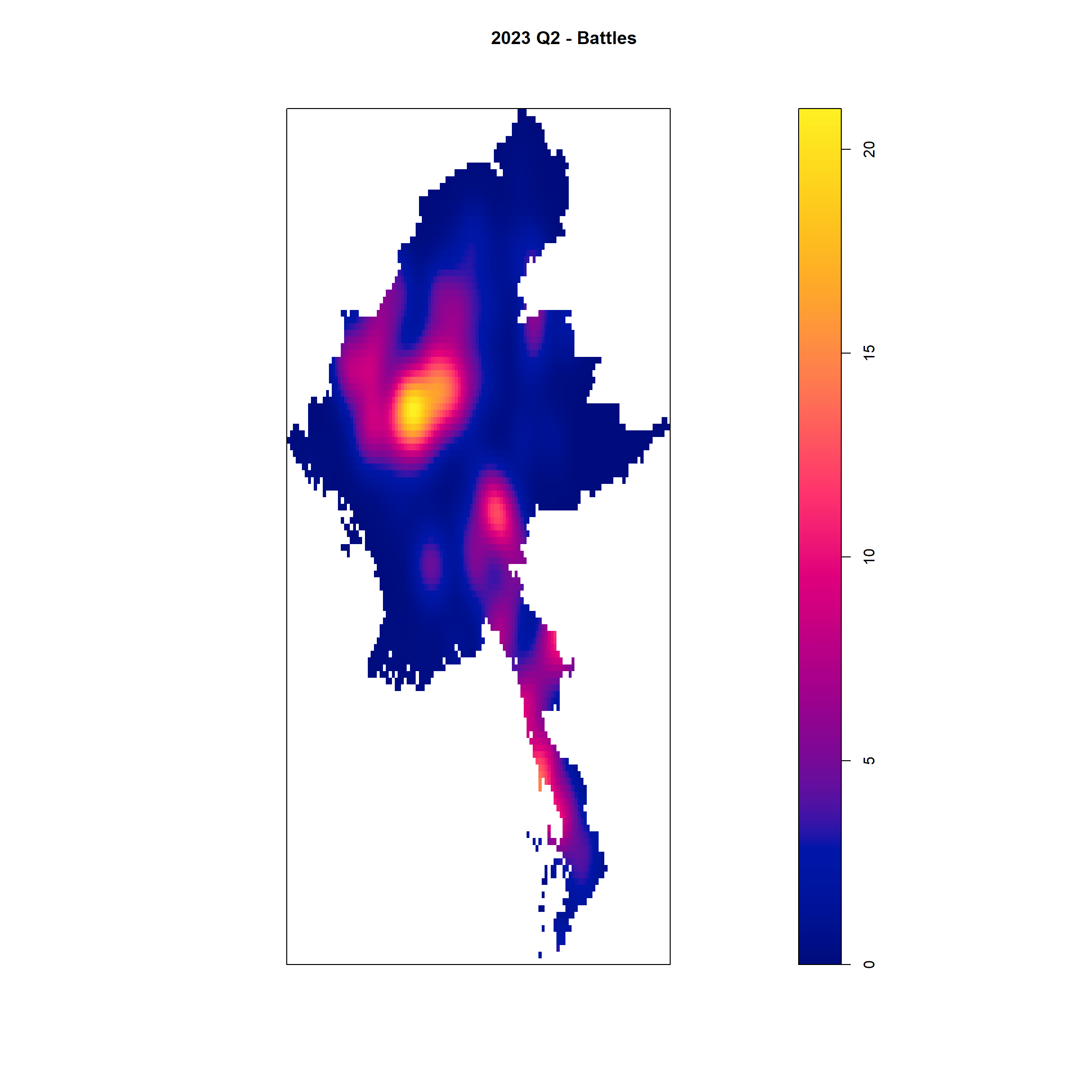
Example <- "Violence against civilians"
my_2023_Q2 <- acled_sf  %>%
  filter(event_type == Example & quarter == "2023 Q2")

write_rds(my_2023_Q2, "data/rds/my_2023_Q2_VAC_quarter_data_regions_sf.rds")

quarter_data <- as_Spatial(my_2023_Q2)
quarter_data_sp <- as(quarter_data, "SpatialPoints")
quarter_data_ppp <- as.ppp(st_coordinates(my_2023_Q2), st_bbox(my_2023_Q2))

quarter_data_ppp_jit <- rjitter(quarter_data_ppp,
                             retry=TRUE,
                             nsim=1,
                             drop=TRUE)
my_2023_Q2_VAC_quarter_data_regions_ppp = quarter_data_ppp_jit[regions_owin]
quarter_data_regions_ppp.km <- rescale.ppp(my_2023_Q2_VAC_quarter_data_regions_ppp, 50000, "km")
bw_scott <- bw.scott(quarter_data_regions_ppp.km)
plot(density(quarter_data_regions_ppp.km,
sigma=bw_scott/2,
edge=TRUE,
kernel="gaussian"),
main = "2023 Q2 - Violence against civilians")
Quarter 3
Example <- "Explosions/Remote violence"
my_2023_Q3 <- acled_sf  %>%
  filter(event_type == Example & quarter == "2023 Q3")

write_rds(my_2023_Q3, "data/rds/my_2023_Q3_ER_quarter_data_regions_sf.rds")

quarter_data <- as_Spatial(my_2023_Q3)
quarter_data_sp <- as(quarter_data, "SpatialPoints")
quarter_data_ppp <- as.ppp(st_coordinates(my_2023_Q3), st_bbox(my_2023_Q3))

quarter_data_ppp_jit <- rjitter(quarter_data_ppp,
                             retry=TRUE,
                             nsim=1,
                             drop=TRUE)
my_2023_Q3_ER_quarter_data_regions_ppp = quarter_data_ppp_jit[regions_owin]
quarter_data_regions_ppp.km <- rescale.ppp(my_2023_Q3_ER_quarter_data_regions_ppp, 50000, "km")
bw_scott <- bw.scott(quarter_data_regions_ppp.km)
plot(density(quarter_data_regions_ppp.km,
sigma=bw_scott/2,
edge=TRUE,
kernel="gaussian"),
main = "2023 Q3 - Explosion/Remote violence")
Example <- "Strategic developments"
my_2023_Q3 <- acled_sf  %>%
  filter(event_type == Example & quarter == "2023 Q3")

write_rds(my_2023_Q3, "data/rds/my_2023_Q3_SD_quarter_data_regions_sf.rds")

quarter_data <- as_Spatial(my_2023_Q3)
quarter_data_sp <- as(quarter_data, "SpatialPoints")
quarter_data_ppp <- as.ppp(st_coordinates(my_2023_Q3), st_bbox(my_2023_Q3))

quarter_data_ppp_jit <- rjitter(quarter_data_ppp,
                             retry=TRUE,
                             nsim=1,
                             drop=TRUE)
my_2023_Q3_SD_quarter_data_regions_ppp = quarter_data_ppp_jit[regions_owin]
quarter_data_regions_ppp.km <- rescale.ppp(my_2023_Q3_SD_quarter_data_regions_ppp, 50000, "km")
bw_scott <- bw.scott(quarter_data_regions_ppp.km)
plot(density(quarter_data_regions_ppp.km,
sigma=bw_scott/2,
edge=TRUE,
kernel="gaussian"),
main = "2023 Q3 - Strategic developments")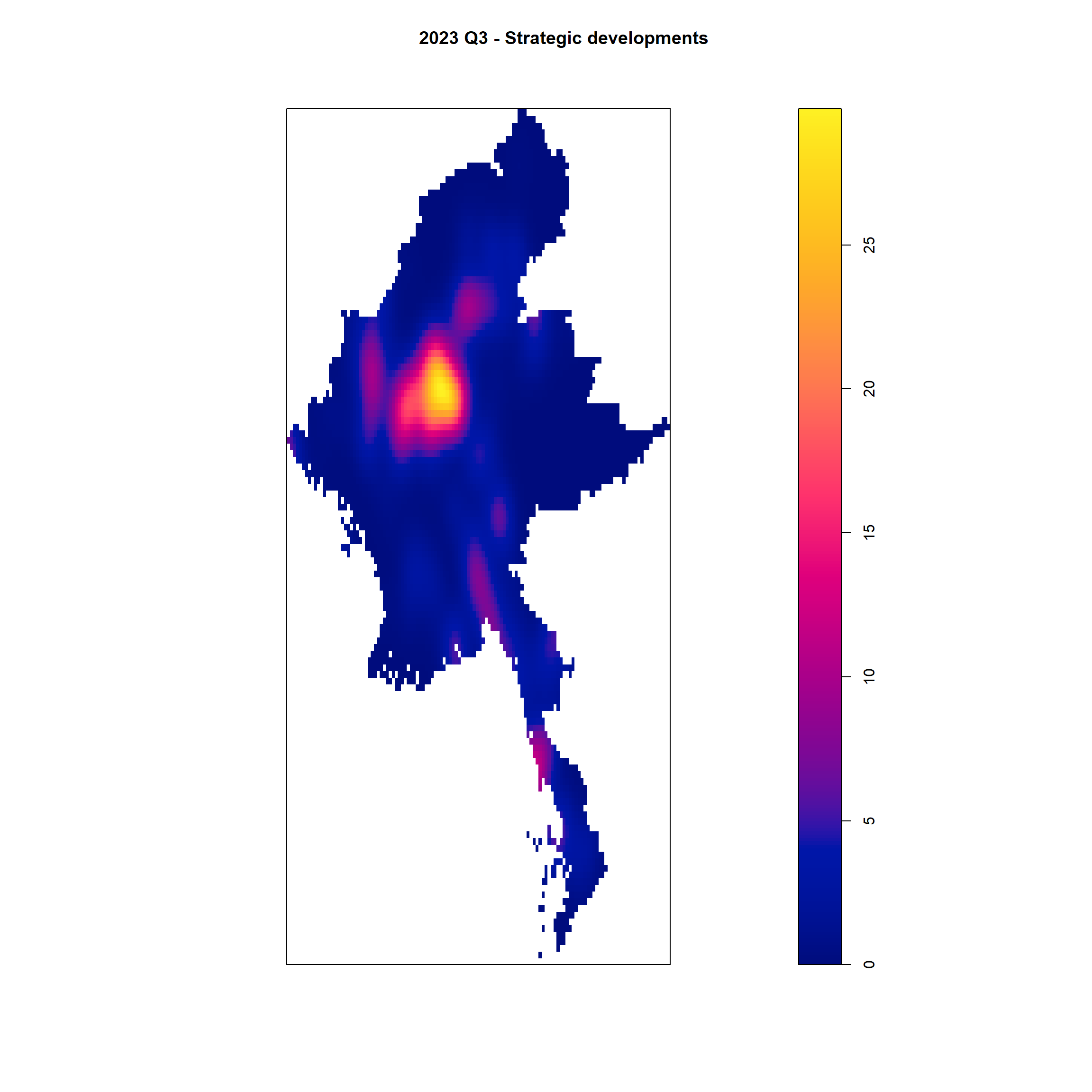
Example <- "Battles"
my_2023_Q3 <- acled_sf  %>%
  filter(event_type == Example & quarter == "2023 Q3")

write_rds(my_2023_Q3, "data/rds/my_2023_Q3_B_quarter_data_regions_sf.rds")

quarter_data <- as_Spatial(my_2023_Q3)
quarter_data_sp <- as(quarter_data, "SpatialPoints")
quarter_data_ppp <- as.ppp(st_coordinates(my_2023_Q3), st_bbox(my_2023_Q3))

quarter_data_ppp_jit <- rjitter(quarter_data_ppp,
                             retry=TRUE,
                             nsim=1,
                             drop=TRUE)
my_2023_Q3_B_quarter_data_regions_ppp = quarter_data_ppp_jit[regions_owin]
quarter_data_regions_ppp.km <- rescale.ppp(my_2023_Q3_B_quarter_data_regions_ppp, 50000, "km")
bw_scott <- bw.scott(quarter_data_regions_ppp.km)
plot(density(quarter_data_regions_ppp.km,
sigma=bw_scott/2,
edge=TRUE,
kernel="gaussian"),
main = "2023 Q3 - Battles")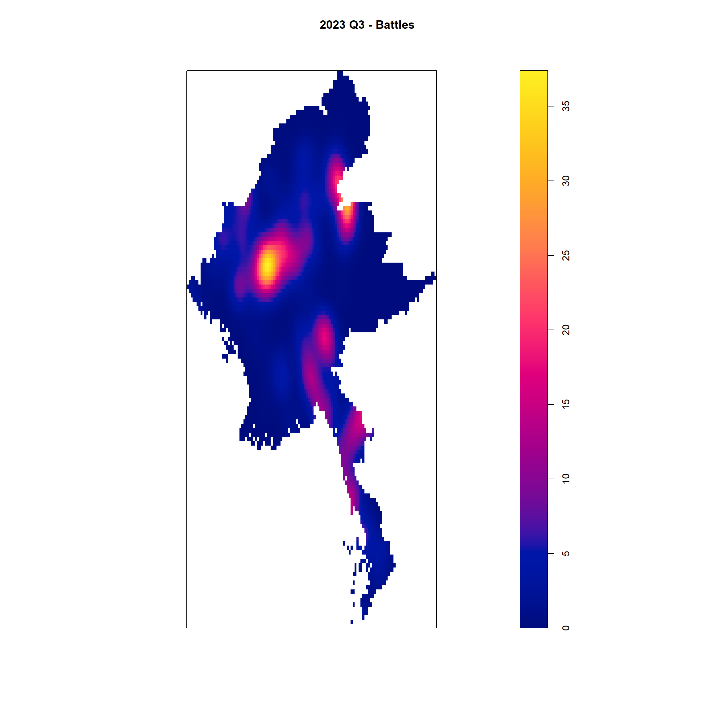
Example <- "Violence against civilians"
my_2023_Q3 <- acled_sf  %>%
  filter(event_type == Example & quarter == "2023 Q3")

write_rds(my_2023_Q3, "data/rds/my_2023_Q3_VAC_quarter_data_regions_sf.rds")

quarter_data <- as_Spatial(my_2023_Q3)
quarter_data_sp <- as(quarter_data, "SpatialPoints")
quarter_data_ppp <- as.ppp(st_coordinates(my_2023_Q3), st_bbox(my_2023_Q3))

quarter_data_ppp_jit <- rjitter(quarter_data_ppp,
                             retry=TRUE,
                             nsim=1,
                             drop=TRUE)
my_2023_Q3_VAC_quarter_data_regions_ppp = quarter_data_ppp_jit[regions_owin]
quarter_data_regions_ppp.km <- rescale.ppp(my_2023_Q3_VAC_quarter_data_regions_ppp, 50000, "km")
bw_scott <- bw.scott(quarter_data_regions_ppp.km)
plot(density(quarter_data_regions_ppp.km,
sigma=bw_scott/2,
edge=TRUE,
kernel="gaussian"),
main = "2023 Q3 - Violence against civilians")
Quarter 4
Example <- "Explosions/Remote violence"
my_2023_Q4 <- acled_sf  %>%
  filter(event_type == Example & quarter == "2023 Q4")

write_rds(my_2023_Q4, "data/rds/my_2023_Q4_ER_quarter_data_regions_sf.rds")

quarter_data <- as_Spatial(my_2023_Q4)
quarter_data_sp <- as(quarter_data, "SpatialPoints")
quarter_data_ppp <- as.ppp(st_coordinates(my_2023_Q4), st_bbox(my_2023_Q4))

quarter_data_ppp_jit <- rjitter(quarter_data_ppp,
                             retry=TRUE,
                             nsim=1,
                             drop=TRUE)
my_2023_Q4_ER_quarter_data_regions_ppp = quarter_data_ppp_jit[regions_owin]
quarter_data_regions_ppp.km <- rescale.ppp(my_2023_Q4_ER_quarter_data_regions_ppp, 50000, "km")
bw_scott <- bw.scott(quarter_data_regions_ppp.km)
plot(density(quarter_data_regions_ppp.km,
sigma=bw_scott/2,
edge=TRUE,
kernel="gaussian"),
main = "2023 Q4 - Explosion/Remote violence")
Example <- "Strategic developments"
my_2023_Q4 <- acled_sf  %>%
  filter(event_type == Example & quarter == "2023 Q4")

write_rds(my_2023_Q4, "data/rds/my_2023_Q4_SD_quarter_data_regions_sf.rds")

quarter_data <- as_Spatial(my_2023_Q4)
quarter_data_sp <- as(quarter_data, "SpatialPoints")
quarter_data_ppp <- as.ppp(st_coordinates(my_2023_Q4), st_bbox(my_2023_Q4))

quarter_data_ppp_jit <- rjitter(quarter_data_ppp,
                             retry=TRUE,
                             nsim=1,
                             drop=TRUE)
my_2023_Q4_SD_quarter_data_regions_ppp = quarter_data_ppp_jit[regions_owin]
quarter_data_regions_ppp.km <- rescale.ppp(my_2023_Q4_SD_quarter_data_regions_ppp, 50000, "km")
bw_scott <- bw.scott(quarter_data_regions_ppp.km)
plot(density(quarter_data_regions_ppp.km,
sigma=bw_scott/2,
edge=TRUE,
kernel="gaussian"),
main = "2023 Q4 - Strategic developments")
Example <- "Battles"
my_2023_Q4 <- acled_sf  %>%
  filter(event_type == Example & quarter == "2023 Q4")

write_rds(my_2023_Q4, "data/rds/my_2023_Q4_B_quarter_data_regions_sf.rds")

quarter_data <- as_Spatial(my_2023_Q4)
quarter_data_sp <- as(quarter_data, "SpatialPoints")
quarter_data_ppp <- as.ppp(st_coordinates(my_2023_Q4), st_bbox(my_2023_Q4))

quarter_data_ppp_jit <- rjitter(quarter_data_ppp,
                             retry=TRUE,
                             nsim=1,
                             drop=TRUE)
my_2023_Q4_B_quarter_data_regions_ppp = quarter_data_ppp_jit[regions_owin]
quarter_data_regions_ppp.km <- rescale.ppp(my_2023_Q4_B_quarter_data_regions_ppp, 50000, "km")
bw_scott <- bw.scott(quarter_data_regions_ppp.km)
plot(density(quarter_data_regions_ppp.km,
sigma=bw_scott/2,
edge=TRUE,
kernel="gaussian"),
main = "2023 Q4 - Battles")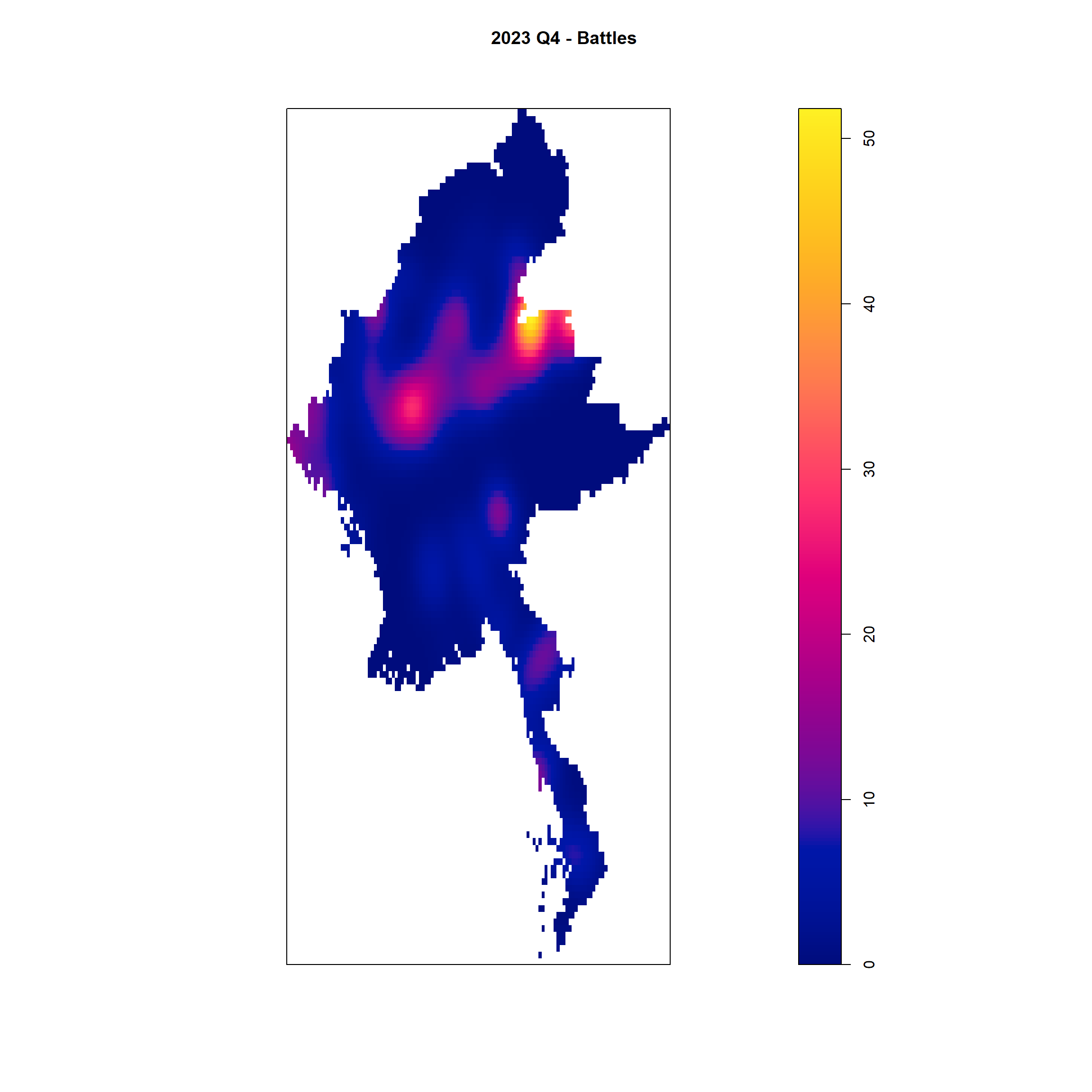
Example <- "Violence against civilians"
my_2023_Q4 <- acled_sf  %>%
  filter(event_type == Example & quarter == "2023 Q4")

write_rds(my_2023_Q4, "data/rds/my_2023_Q4_VAC_quarter_data_regions_sf.rds")

quarter_data <- as_Spatial(my_2023_Q4)
quarter_data_sp <- as(quarter_data, "SpatialPoints")
quarter_data_ppp <- as.ppp(st_coordinates(my_2023_Q4), st_bbox(my_2023_Q4))

quarter_data_ppp_jit <- rjitter(quarter_data_ppp,
                             retry=TRUE,
                             nsim=1,
                             drop=TRUE)
my_2023_Q4_VAC_quarter_data_regions_ppp = quarter_data_ppp_jit[regions_owin]
quarter_data_regions_ppp.km <- rescale.ppp(my_2023_Q4_VAC_quarter_data_regions_ppp, 50000, "km")
bw_scott <- bw.scott(quarter_data_regions_ppp.km)
plot(density(quarter_data_regions_ppp.km,
sigma=bw_scott/2,
edge=TRUE,
kernel="gaussian"),
main = "2023 Q4 - Violence against civilians")
Year 2024
Quarter 1
Example <- "Explosions/Remote violence"
my_2024_Q1 <- acled_sf  %>%
  filter(event_type == Example & quarter == "2024 Q1")

write_rds(my_2024_Q1, "data/rds/my_2024_Q1_ER_quarter_data_regions_sf.rds")

quarter_data <- as_Spatial(my_2024_Q1)
quarter_data_sp <- as(quarter_data, "SpatialPoints")
quarter_data_ppp <- as.ppp(st_coordinates(my_2024_Q1), st_bbox(my_2024_Q1))

quarter_data_ppp_jit <- rjitter(quarter_data_ppp,
                             retry=TRUE,
                             nsim=1,
                             drop=TRUE)
my_2024_Q1_ER_quarter_data_regions_ppp = quarter_data_ppp_jit[regions_owin]
quarter_data_regions_ppp.km <- rescale.ppp(my_2024_Q1_ER_quarter_data_regions_ppp, 50000, "km")
bw_scott <- bw.scott(quarter_data_regions_ppp.km)
plot(density(quarter_data_regions_ppp.km,
sigma=bw_scott/2,
edge=TRUE,
kernel="gaussian"),
main = "2024 Q1 - Explosion/Remote violence")
Example <- "Strategic developments"
my_2024_Q1 <- acled_sf  %>%
  filter(event_type == Example & quarter == "2024 Q1")

write_rds(my_2024_Q1, "data/rds/my_2024_Q1_SD_quarter_data_regions_sf.rds")

quarter_data <- as_Spatial(my_2024_Q1)
quarter_data_sp <- as(quarter_data, "SpatialPoints")
quarter_data_ppp <- as.ppp(st_coordinates(my_2024_Q1), st_bbox(my_2024_Q1))

quarter_data_ppp_jit <- rjitter(quarter_data_ppp,
                             retry=TRUE,
                             nsim=1,
                             drop=TRUE)
my_2024_Q1_SD_quarter_data_regions_ppp = quarter_data_ppp_jit[regions_owin]
quarter_data_regions_ppp.km <- rescale.ppp(my_2024_Q1_SD_quarter_data_regions_ppp, 50000, "km")
bw_scott <- bw.scott(quarter_data_regions_ppp.km)
plot(density(quarter_data_regions_ppp.km,
sigma=bw_scott/2,
edge=TRUE,
kernel="gaussian"),
main = "2024 Q1 - Strategic developments")
Example <- "Battles"
my_2024_Q1 <- acled_sf  %>%
  filter(event_type == Example & quarter == "2024 Q1")

write_rds(my_2024_Q1, "data/rds/my_2024_Q1_B_quarter_data_regions_sf.rds")

quarter_data <- as_Spatial(my_2024_Q1)
quarter_data_sp <- as(quarter_data, "SpatialPoints")
quarter_data_ppp <- as.ppp(st_coordinates(my_2024_Q1), st_bbox(my_2024_Q1))

quarter_data_ppp_jit <- rjitter(quarter_data_ppp,
                             retry=TRUE,
                             nsim=1,
                             drop=TRUE)
my_2024_Q1_B_quarter_data_regions_ppp = quarter_data_ppp_jit[regions_owin]
quarter_data_regions_ppp.km <- rescale.ppp(my_2024_Q1_B_quarter_data_regions_ppp, 50000, "km")
bw_scott <- bw.scott(quarter_data_regions_ppp.km)
plot(density(quarter_data_regions_ppp.km,
sigma=bw_scott/2,
edge=TRUE,
kernel="gaussian"),
main = "2024 Q1 - Battles")
Example <- "Violence against civilians"
my_2024_Q1 <- acled_sf  %>%
  filter(event_type == Example & quarter == "2024 Q1")

write_rds(my_2024_Q1, "data/rds/my_2024_Q1_VAC_quarter_data_regions_sf.rds")

quarter_data <- as_Spatial(my_2024_Q1)
quarter_data_sp <- as(quarter_data, "SpatialPoints")
quarter_data_ppp <- as.ppp(st_coordinates(my_2024_Q1), st_bbox(my_2024_Q1))

quarter_data_ppp_jit <- rjitter(quarter_data_ppp,
                             retry=TRUE,
                             nsim=1,
                             drop=TRUE)
my_2024_Q1_VAC_quarter_data_regions_ppp = quarter_data_ppp_jit[regions_owin]
quarter_data_regions_ppp.km <- rescale.ppp(my_2024_Q1_VAC_quarter_data_regions_ppp, 50000, "km")
bw_scott <- bw.scott(quarter_data_regions_ppp.km)
plot(density(quarter_data_regions_ppp.km,
sigma=bw_scott/2,
edge=TRUE,
kernel="gaussian"),
main = "2024 Q1 -Violence against civilians")
Quarter 2
Example <- "Explosions/Remote violence"
my_2024_Q2 <- acled_sf  %>%
  filter(event_type == Example & quarter == "2024 Q2")

write_rds(my_2024_Q2, "data/rds/my_2024_Q2_ER_quarter_data_regions_sf.rds")

quarter_data <- as_Spatial(my_2024_Q2)
quarter_data_sp <- as(quarter_data, "SpatialPoints")
quarter_data_ppp <- as.ppp(st_coordinates(my_2024_Q2), st_bbox(my_2024_Q2))

quarter_data_ppp_jit <- rjitter(quarter_data_ppp,
                             retry=TRUE,
                             nsim=1,
                             drop=TRUE)
my_2024_Q2_ER_quarter_data_regions_ppp = quarter_data_ppp_jit[regions_owin]
quarter_data_regions_ppp.km <- rescale.ppp(my_2024_Q2_ER_quarter_data_regions_ppp, 50000, "km")
bw_scott <- bw.scott(quarter_data_regions_ppp.km)
plot(density(quarter_data_regions_ppp.km,
sigma=bw_scott/2,
edge=TRUE,
kernel="gaussian"),
main = "2024 Q2 - Explosion/Remote violence")
Example <- "Strategic developments"
my_2024_Q2 <- acled_sf  %>%
  filter(event_type == Example & quarter == "2024 Q2")

write_rds(my_2024_Q2, "data/rds/my_2024_Q2_SD_quarter_data_regions_sf.rds")

quarter_data <- as_Spatial(my_2024_Q2)
quarter_data_sp <- as(quarter_data, "SpatialPoints")
quarter_data_ppp <- as.ppp(st_coordinates(my_2024_Q2), st_bbox(my_2024_Q2))

quarter_data_ppp_jit <- rjitter(quarter_data_ppp,
                             retry=TRUE,
                             nsim=1,
                             drop=TRUE)
my_2024_Q2_SD_quarter_data_regions_ppp = quarter_data_ppp_jit[regions_owin]
quarter_data_regions_ppp.km <- rescale.ppp(my_2024_Q2_SD_quarter_data_regions_ppp, 50000, "km")
bw_scott <- bw.scott(quarter_data_regions_ppp.km)
plot(density(quarter_data_regions_ppp.km,
sigma=bw_scott/2,
edge=TRUE,
kernel="gaussian"),
main = "2024 Q2 - Strategic developments")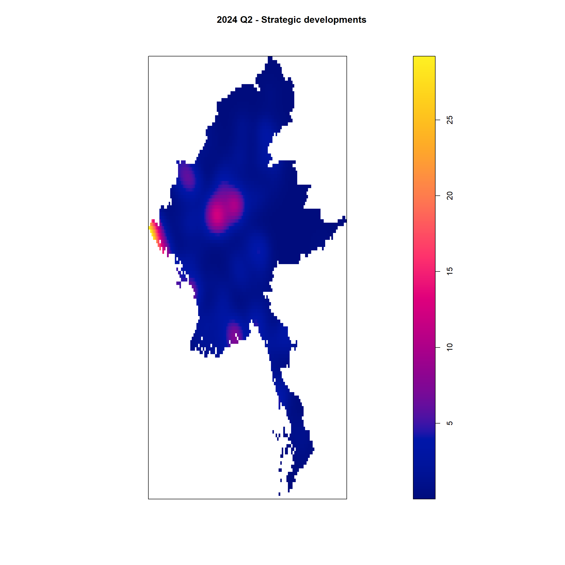
Example <- "Battles"
my_2024_Q2 <- acled_sf  %>%
  filter(event_type == Example & quarter == "2024 Q2")

write_rds(my_2024_Q2, "data/rds/my_2024_Q2_B_quarter_data_regions_sf.rds")

quarter_data <- as_Spatial(my_2024_Q2)
quarter_data_sp <- as(quarter_data, "SpatialPoints")
quarter_data_ppp <- as.ppp(st_coordinates(my_2024_Q2), st_bbox(my_2024_Q2))

quarter_data_ppp_jit <- rjitter(quarter_data_ppp,
                             retry=TRUE,
                             nsim=1,
                             drop=TRUE)
my_2024_Q2_B_quarter_data_regions_ppp = quarter_data_ppp_jit[regions_owin]
quarter_data_regions_ppp.km <- rescale.ppp(my_2024_Q2_B_quarter_data_regions_ppp, 50000, "km")
bw_scott <- bw.scott(quarter_data_regions_ppp.km)
plot(density(quarter_data_regions_ppp.km,
sigma=bw_scott/2,
edge=TRUE,
kernel="gaussian"),
main = "2024 Q2 - Battles")
Example <- "Violence against civilians"
my_2024_Q2 <- acled_sf  %>%
  filter(event_type == Example & quarter == "2024 Q2")

write_rds(my_2024_Q2, "data/rds/my_2024_Q2_VAC_quarter_data_regions_sf.rds")

quarter_data <- as_Spatial(my_2024_Q2)
quarter_data_sp <- as(quarter_data, "SpatialPoints")
quarter_data_ppp <- as.ppp(st_coordinates(my_2024_Q2), st_bbox(my_2024_Q2))

quarter_data_ppp_jit <- rjitter(quarter_data_ppp,
                             retry=TRUE,
                             nsim=1,
                             drop=TRUE)
my_2024_Q2_VAC_quarter_data_regions_ppp = quarter_data_ppp_jit[regions_owin]
quarter_data_regions_ppp.km <- rescale.ppp(my_2024_Q2_VAC_quarter_data_regions_ppp, 50000, "km")
bw_scott <- bw.scott(quarter_data_regions_ppp.km)
plot(density(quarter_data_regions_ppp.km,
sigma=bw_scott/2,
edge=TRUE,
kernel="gaussian"),
main = "2024 Q2 - Violence against civilians")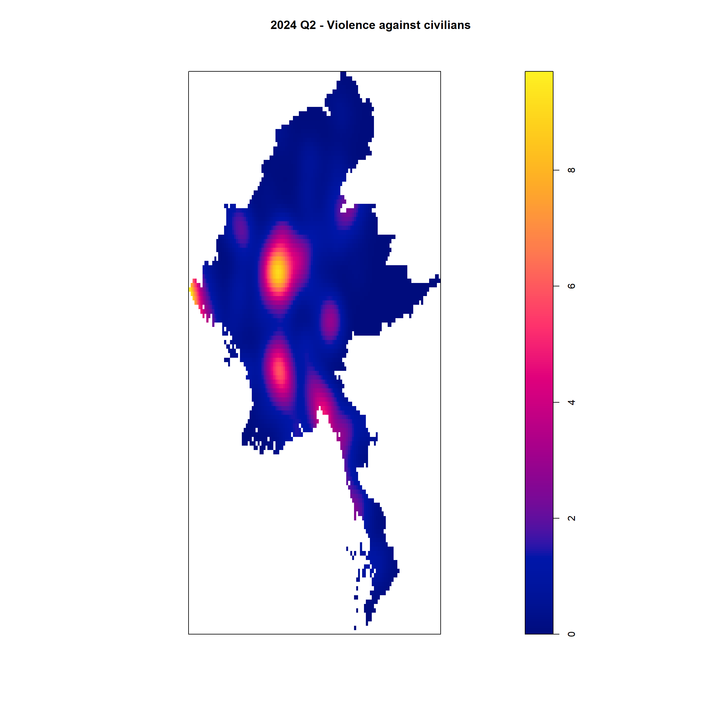
1.6 2nd-Order Spatial Point Patterns Analysis
1.6.1 Overview
To perform a Second-order Spatial Point Patterns Analysis, we utilize the G, F, K, and L functions of the spatstat package in R. Each of these functions analyzes different aspects of spatial point patterns. Given the nature of the dataset, it is crucial to choose an analysis that best captures the complexity of spatial distributions for conflict events. Each of the spatial functions (G, F, K, and L) has its strengths, but here’s how they align with conflict data analysis, with a particular focus on the G-function:
G-Function (Nearest Neighbor Distribution):
- Detecting local clustering: The G-function focuses on the distribution of nearest neighbors, making it particularly useful for detecting local clustering of events. In the civil war context, where conflict events often cluster in specific regions or around key areas of interest (e.g., cities, roads, military bases), the G-function can quickly and efficiently help identify hotspots of violence. Its simplicity and computational efficiency make it an excellent choice for analyzing localized patterns of violence, especially when time and resources are limited.
F-Function (Empty Space Function):
- Detecting global regularity: The F-function measures the distance from random locations to the nearest event. While it can offer insights into the global spread of events, this function is less relevant for conflict analysis because it emphasizes regularity over clustering, which is not typical in conflict zones. Conflict events are rarely evenly spaced, making the F-function less suited for this kind of data.
K-Function (Ripley’s K-Function):
- Multi-scale clustering: The K-function is valuable for analyzing clustering at different spatial scales, especially in hierarchical conflict scenarios where regional and local clusters coexist. However, the K-function’s multi-scale nature comes with a higher computational cost, making it less practical for when large datasets are involved. While informative, its complexity and runtime can be a drawback.
L-Function (Transformed K-Function):
- Simplifying K-function results: The L-function is a linearized version of the K-function and offers more intuitive interpretations of clustering versus dispersion. However, like the K-function, it involves significant computation time, and its added complexity may not always justify its use, especially when the G-function already provides key insights into local clustering.
Given the nature of the civil war event data, where localized patterns and hotspots of violence are of primary concern, the G-function emerges as the most suitable tool for analysis. Its ability to efficiently detect local clustering while being computationally lightweight makes it a clear choice. While both K-function and L-functions offer multi-scale insights, they come at the cost of significant computation time, which may not be necessary for this analysis.
The G-function provides a focused and practical approach to understanding the spatial distribution of conflict events, making it the preferred choice in this context.
Note
Due to the non-deterministic nature of running each simulation, the set.seed() function is employed to ensure the reproducibility of the simulation results. This is especially important for lower values of nsim, as it helps mitigate the random variability inherent in smaller sample sizes. By using a fixed seed, the analysis produces consistent outcomes across repeated runs, allowing for reliable comparisons and interpretations.
This approach enables us to assess whether the observed spatial point patterns significantly deviate from randomness. By simulating random point processes and comparing them to the observed data, we can identify potential clustering or dispersion patterns. These insights are critical in understanding the underlying structure of armed conflict events over time, helping to reveal whether the events are influenced by specific geographic or temporal factors or if they occur more randomly.
The results of this analysis contribute to a deeper understanding of the spatial-temporal dynamics of armed conflict, such as hotspots of violence, escalation patterns, and event diffusion across regions. This information is invaluable for conflict analysis, policy-making, and intervention planning.
Explosions/Remote violence overview
set.seed(123)

# Create a list of all the ER quarter datasets
er_datasets <- list(
  my_2021_Q1_ER_quarter_data_regions_ppp,
  my_2021_Q2_ER_quarter_data_regions_ppp,
  my_2021_Q3_ER_quarter_data_regions_ppp,
  my_2021_Q4_ER_quarter_data_regions_ppp,
  my_2022_Q1_ER_quarter_data_regions_ppp,
  my_2022_Q2_ER_quarter_data_regions_ppp,
  my_2022_Q3_ER_quarter_data_regions_ppp,
  my_2022_Q4_ER_quarter_data_regions_ppp,
  my_2023_Q1_ER_quarter_data_regions_ppp,
  my_2023_Q2_ER_quarter_data_regions_ppp,
  my_2023_Q3_ER_quarter_data_regions_ppp,
  my_2023_Q4_ER_quarter_data_regions_ppp,
  my_2024_Q1_ER_quarter_data_regions_ppp,
  my_2024_Q2_ER_quarter_data_regions_ppp
)

# Corresponding year and quarter labels for the plots
er_labels <- c(
  "2021 Q1", "2021 Q2", "2021 Q3", "2021 Q4",
  "2022 Q1", "2022 Q2", "2022 Q3", "2022 Q4",
  "2023 Q1", "2023 Q2", "2023 Q3", "2023 Q4",
  "2024 Q1", "2024 Q2"
)

# Set up the plotting area
par(mar = c(2,0,2,0))
par(mfrow=c(4,4))

# Loop through each dataset and create the KDE plots
for (i in seq_along(er_datasets)) {
    G_CK.csr <- envelope(er_datasets[[i]], Gest, nsim = 50, correction="all", parallel = parallel::detectCores()
    )
  plot(G_CK.csr, xlim=c(0,10000), main= er_labels[[i]])
}
Generating 50 simulations of CSR ...
1, 2, 3, 4, 5, 6, 7, 8, 9, 10, 11, 12, 13, 14, 15, 16, 17, 18, 19, 20,
21, 22, 23, 24, 25, 26, 27, 28, 29, 30, 31, 32, 33, 34, 35, 36, 37, 38, 39, 40,
41, 42, 43, 44, 45, 46, 47, 48, 49,
50.
Done.Generating 50 simulations of CSR ...
1, 2, 3, 4, 5, 6, 7, 8, 9, 10, 11, 12, 13, 14, 15, 16, 17, 18, 19, 20,
21, 22, 23, 24, 25, 26, 27, 28, 29, 30, 31, 32, 33, 34, 35, 36, 37, 38, 39, 40,
41, 42, 43, 44, 45, 46, 47, 48, 49,
50.
Done.Generating 50 simulations of CSR ...
1, 2, 3, 4, 5, 6, 7, 8, 9, 10, 11, 12, 13, 14, 15, 16, 17, 18, 19, 20,
21, 22, 23, 24, 25, 26, 27, 28, 29, 30, 31, 32, 33, 34, 35, 36, 37, 38, 39, 40,
41, 42, 43, 44, 45, 46, 47, 48, 49,
50.
Done.Generating 50 simulations of CSR ...
1, 2, 3, 4, 5, 6, 7, 8, 9, 10, 11, 12, 13, 14, 15, 16, 17, 18, 19, 20,
21, 22, 23, 24, 25, 26, 27, 28, 29, 30, 31, 32, 33, 34, 35, 36, 37, 38, 39, 40,
41, 42, 43, 44, 45, 46, 47, 48, 49,
50.
Done.Generating 50 simulations of CSR ...
1, 2, 3, 4, 5, 6, 7, 8, 9, 10, 11, 12, 13, 14, 15, 16, 17, 18, 19, 20,
21, 22, 23, 24, 25, 26, 27, 28, 29, 30, 31, 32, 33, 34, 35, 36, 37, 38, 39, 40,
41, 42, 43, 44, 45, 46, 47, 48, 49,
50.
Done.Generating 50 simulations of CSR ...
1, 2, 3, 4, 5, 6, 7, 8, 9, 10, 11, 12, 13, 14, 15, 16, 17, 18, 19, 20,
21, 22, 23, 24, 25, 26, 27, 28, 29, 30, 31, 32, 33, 34, 35, 36, 37, 38, 39, 40,
41, 42, 43, 44, 45, 46, 47, 48, 49,
50.
Done.Generating 50 simulations of CSR ...
1, 2, 3, 4, 5, 6, 7, 8, 9, 10, 11, 12, 13, 14, 15, 16, 17, 18, 19, 20,
21, 22, 23, 24, 25, 26, 27, 28, 29, 30, 31, 32, 33, 34, 35, 36, 37, 38, 39, 40,
41, 42, 43, 44, 45, 46, 47, 48, 49,
50.
Done.Generating 50 simulations of CSR ...
1, 2, 3, 4, 5, 6, 7, 8, 9, 10, 11, 12, 13, 14, 15, 16, 17, 18, 19, 20,
21, 22, 23, 24, 25, 26, 27, 28, 29, 30, 31, 32, 33, 34, 35, 36, 37, 38, 39, 40,
41, 42, 43, 44, 45, 46, 47, 48, 49,
50.
Done.Generating 50 simulations of CSR ...
1, 2, 3, 4, 5, 6, 7, 8, 9, 10, 11, 12, 13, 14, 15, 16, 17, 18, 19, 20,
21, 22, 23, 24, 25, 26, 27, 28, 29, 30, 31, 32, 33, 34, 35, 36, 37, 38, 39, 40,
41, 42, 43, 44, 45, 46, 47, 48, 49,
50.
Done.Generating 50 simulations of CSR ...
1, 2, 3, 4, 5, 6, 7, 8, 9, 10, 11, 12, 13, 14, 15, 16, 17, 18, 19, 20,
21, 22, 23, 24, 25, 26, 27, 28, 29, 30, 31, 32, 33, 34, 35, 36, 37, 38, 39, 40,
41, 42, 43, 44, 45, 46, 47, 48, 49,
50.
Done.Generating 50 simulations of CSR ...
1, 2, 3, 4, 5, 6, 7, 8, 9, 10, 11, 12, 13, 14, 15, 16, 17, 18, 19, 20,
21, 22, 23, 24, 25, 26, 27, 28, 29, 30, 31, 32, 33, 34, 35, 36, 37, 38, 39, 40,
41, 42, 43, 44, 45, 46, 47, 48, 49,
50.
Done.Generating 50 simulations of CSR ...
1, 2, 3, 4, 5, 6, 7, 8, 9, 10, 11, 12, 13, 14, 15, 16, 17, 18, 19, 20,
21, 22, 23, 24, 25, 26, 27, 28, 29, 30, 31, 32, 33, 34, 35, 36, 37, 38, 39, 40,
41, 42, 43, 44, 45, 46, 47, 48, 49,
50.
Done.Generating 50 simulations of CSR ...
1, 2, 3, 4, 5, 6, 7, 8, 9, 10, 11, 12, 13, 14, 15, 16, 17, 18, 19, 20,
21, 22, 23, 24, 25, 26, 27, 28, 29, 30, 31, 32, 33, 34, 35, 36, 37, 38, 39, 40,
41, 42, 43, 44, 45, 46, 47, 48, 49,
50.
Done.Generating 50 simulations of CSR ...
1, 2, 3, 4, 5, 6, 7, 8, 9, 10, 11, 12, 13, 14, 15, 16, 17, 18, 19, 20,
21, 22, 23, 24, 25, 26, 27, 28, 29, 30, 31, 32, 33, 34, 35, 36, 37, 38, 39, 40,
41, 42, 43, 44, 45, 46, 47, 48, 49,
50.
Done.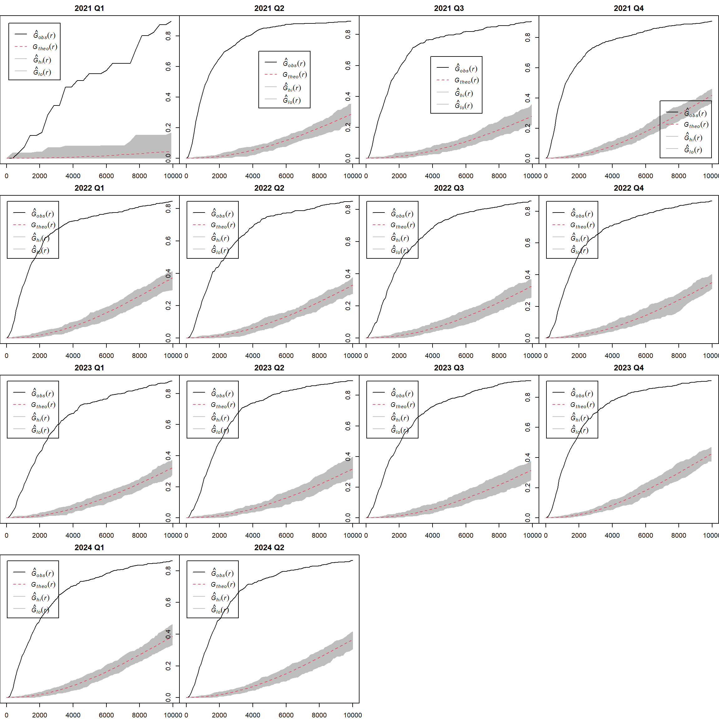
Strategic developments overview
set.seed(124)

# Create a list of all the ER quarter datasets
er_datasets <- list(
  my_2021_Q1_SD_quarter_data_regions_ppp,
  my_2021_Q2_SD_quarter_data_regions_ppp,
  my_2021_Q3_SD_quarter_data_regions_ppp,
  my_2021_Q4_SD_quarter_data_regions_ppp,
  my_2022_Q1_SD_quarter_data_regions_ppp,
  my_2022_Q2_SD_quarter_data_regions_ppp,
  my_2022_Q3_SD_quarter_data_regions_ppp,
  my_2022_Q4_SD_quarter_data_regions_ppp,
  my_2023_Q1_SD_quarter_data_regions_ppp,
  my_2023_Q2_SD_quarter_data_regions_ppp,
  my_2023_Q3_SD_quarter_data_regions_ppp,
  my_2023_Q4_SD_quarter_data_regions_ppp,
  my_2024_Q1_SD_quarter_data_regions_ppp,
  my_2024_Q2_SD_quarter_data_regions_ppp
)

# Corresponding year and quarter labels for the plots
er_labels <- c(
  "2021 Q1", "2021 Q2", "2021 Q3", "2021 Q4",
  "2022 Q1", "2022 Q2", "2022 Q3", "2022 Q4",
  "2023 Q1", "2023 Q2", "2023 Q3", "2023 Q4",
  "2024 Q1", "2024 Q2"
)

# Set up the plotting area
par(mar = c(2,1,2,1))
par(mfrow=c(4,4))

# Loop through each dataset and create the KDE plots
for (i in seq_along(er_datasets)) {
    G_CK.csr <- envelope(er_datasets[[i]], Gest, nsim = 50, parallel = parallel::detectCores())
  plot(G_CK.csr, xlim=c(0,10000), main= er_labels[[i]])
}
Generating 50 simulations of CSR ...
1, 2, 3, 4, 5, 6, 7, 8, 9, 10, 11, 12, 13, 14, 15, 16, 17, 18, 19, 20,
21, 22, 23, 24, 25, 26, 27, 28, 29, 30, 31, 32, 33, 34, 35, 36, 37, 38, 39, 40,
41, 42, 43, 44, 45, 46, 47, 48, 49,
50.
Done.Generating 50 simulations of CSR ...
1, 2, 3, 4, 5, 6, 7, 8, 9, 10, 11, 12, 13, 14, 15, 16, 17, 18, 19, 20,
21, 22, 23, 24, 25, 26, 27, 28, 29, 30, 31, 32, 33, 34, 35, 36, 37, 38, 39, 40,
41, 42, 43, 44, 45, 46, 47, 48, 49,
50.
Done.Generating 50 simulations of CSR ...
1, 2, 3, 4, 5, 6, 7, 8, 9, 10, 11, 12, 13, 14, 15, 16, 17, 18, 19, 20,
21, 22, 23, 24, 25, 26, 27, 28, 29, 30, 31, 32, 33, 34, 35, 36, 37, 38, 39, 40,
41, 42, 43, 44, 45, 46, 47, 48, 49,
50.
Done.Generating 50 simulations of CSR ...
1, 2, 3, 4, 5, 6, 7, 8, 9, 10, 11, 12, 13, 14, 15, 16, 17, 18, 19, 20,
21, 22, 23, 24, 25, 26, 27, 28, 29, 30, 31, 32, 33, 34, 35, 36, 37, 38, 39, 40,
41, 42, 43, 44, 45, 46, 47, 48, 49,
50.
Done.Generating 50 simulations of CSR ...
1, 2, 3, 4, 5, 6, 7, 8, 9, 10, 11, 12, 13, 14, 15, 16, 17, 18, 19, 20,
21, 22, 23, 24, 25, 26, 27, 28, 29, 30, 31, 32, 33, 34, 35, 36, 37, 38, 39, 40,
41, 42, 43, 44, 45, 46, 47, 48, 49,
50.
Done.Generating 50 simulations of CSR ...
1, 2, 3, 4, 5, 6, 7, 8, 9, 10, 11, 12, 13, 14, 15, 16, 17, 18, 19, 20,
21, 22, 23, 24, 25, 26, 27, 28, 29, 30, 31, 32, 33, 34, 35, 36, 37, 38, 39, 40,
41, 42, 43, 44, 45, 46, 47, 48, 49,
50.
Done.Generating 50 simulations of CSR ...
1, 2, 3, 4, 5, 6, 7, 8, 9, 10, 11, 12, 13, 14, 15, 16, 17, 18, 19, 20,
21, 22, 23, 24, 25, 26, 27, 28, 29, 30, 31, 32, 33, 34, 35, 36, 37, 38, 39, 40,
41, 42, 43, 44, 45, 46, 47, 48, 49,
50.
Done.Generating 50 simulations of CSR ...
1, 2, 3, 4, 5, 6, 7, 8, 9, 10, 11, 12, 13, 14, 15, 16, 17, 18, 19, 20,
21, 22, 23, 24, 25, 26, 27, 28, 29, 30, 31, 32, 33, 34, 35, 36, 37, 38, 39, 40,
41, 42, 43, 44, 45, 46, 47, 48, 49,
50.
Done.Generating 50 simulations of CSR ...
1, 2, 3, 4, 5, 6, 7, 8, 9, 10, 11, 12, 13, 14, 15, 16, 17, 18, 19, 20,
21, 22, 23, 24, 25, 26, 27, 28, 29, 30, 31, 32, 33, 34, 35, 36, 37, 38, 39, 40,
41, 42, 43, 44, 45, 46, 47, 48, 49,
50.
Done.Generating 50 simulations of CSR ...
1, 2, 3, 4, 5, 6, 7, 8, 9, 10, 11, 12, 13, 14, 15, 16, 17, 18, 19, 20,
21, 22, 23, 24, 25, 26, 27, 28, 29, 30, 31, 32, 33, 34, 35, 36, 37, 38, 39, 40,
41, 42, 43, 44, 45, 46, 47, 48, 49,
50.
Done.Generating 50 simulations of CSR ...
1, 2, 3, 4, 5, 6, 7, 8, 9, 10, 11, 12, 13, 14, 15, 16, 17, 18, 19, 20,
21, 22, 23, 24, 25, 26, 27, 28, 29, 30, 31, 32, 33, 34, 35, 36, 37, 38, 39, 40,
41, 42, 43, 44, 45, 46, 47, 48, 49,
50.
Done.Generating 50 simulations of CSR ...
1, 2, 3, 4, 5, 6, 7, 8, 9, 10, 11, 12, 13, 14, 15, 16, 17, 18, 19, 20,
21, 22, 23, 24, 25, 26, 27, 28, 29, 30, 31, 32, 33, 34, 35, 36, 37, 38, 39, 40,
41, 42, 43, 44, 45, 46, 47, 48, 49,
50.
Done.Generating 50 simulations of CSR ...
1, 2, 3, 4, 5, 6, 7, 8, 9, 10, 11, 12, 13, 14, 15, 16, 17, 18, 19, 20,
21, 22, 23, 24, 25, 26, 27, 28, 29, 30, 31, 32, 33, 34, 35, 36, 37, 38, 39, 40,
41, 42, 43, 44, 45, 46, 47, 48, 49,
50.
Done.Generating 50 simulations of CSR ...
1, 2, 3, 4, 5, 6, 7, 8, 9, 10, 11, 12, 13, 14, 15, 16, 17, 18, 19, 20,
21, 22, 23, 24, 25, 26, 27, 28, 29, 30, 31, 32, 33, 34, 35, 36, 37, 38, 39, 40,
41, 42, 43, 44, 45, 46, 47, 48, 49,
50.
Done.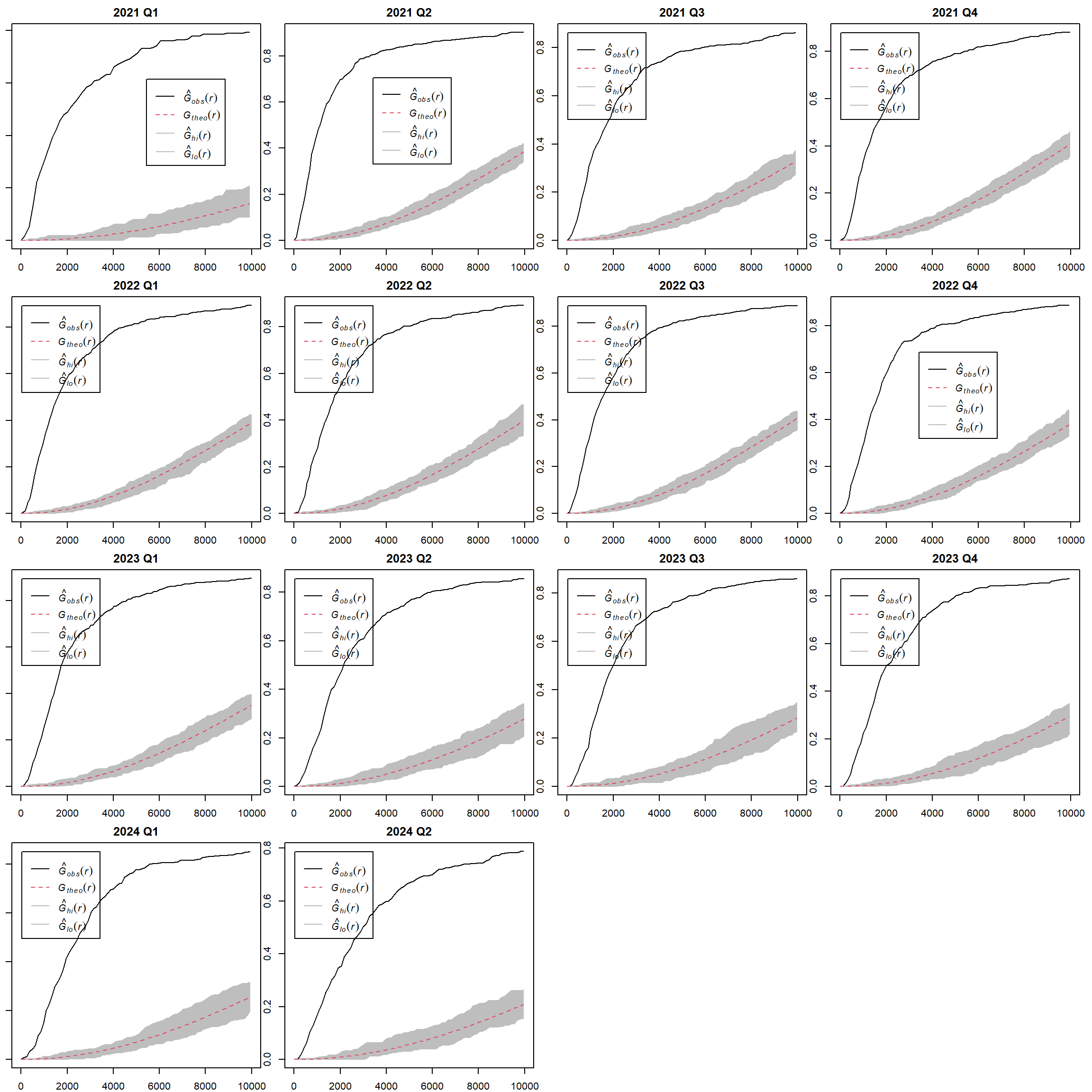
Battles overview
set.seed(125)

# Create a list of all the ER quarter datasets
er_datasets <- list(
  my_2021_Q1_B_quarter_data_regions_ppp,
  my_2021_Q2_B_quarter_data_regions_ppp,
  my_2021_Q3_B_quarter_data_regions_ppp,
  my_2021_Q4_B_quarter_data_regions_ppp,
  my_2022_Q1_B_quarter_data_regions_ppp,
  my_2022_Q2_B_quarter_data_regions_ppp,
  my_2022_Q3_B_quarter_data_regions_ppp,
  my_2022_Q4_B_quarter_data_regions_ppp,
  my_2023_Q1_B_quarter_data_regions_ppp,
  my_2023_Q2_B_quarter_data_regions_ppp,
  my_2023_Q3_B_quarter_data_regions_ppp,
  my_2023_Q4_B_quarter_data_regions_ppp,
  my_2024_Q1_B_quarter_data_regions_ppp,
  my_2024_Q2_B_quarter_data_regions_ppp
)

# Corresponding year and quarter labels for the plots
er_labels <- c(
  "2021 Q1", "2021 Q2", "2021 Q3", "2021 Q4",
  "2022 Q1", "2022 Q2", "2022 Q3", "2022 Q4",
  "2023 Q1", "2023 Q2", "2023 Q3", "2023 Q4",
  "2024 Q1", "2024 Q2"
)

# Set up the plotting area
par(mar = c(2,1,2,1))
par(mfrow=c(4,4))

# Loop through each dataset and create the KDE plots
for (i in seq_along(er_datasets)) {
    G_CK.csr <- envelope(er_datasets[[i]], Gest, nsim = 50, parallel = parallel::detectCores())
  plot(G_CK.csr, xlim=c(0,10000), main= er_labels[[i]])
}
Generating 50 simulations of CSR ...
1, 2, 3, 4, 5, 6, 7, 8, 9, 10, 11, 12, 13, 14, 15, 16, 17, 18, 19, 20,
21, 22, 23, 24, 25, 26, 27, 28, 29, 30, 31, 32, 33, 34, 35, 36, 37, 38, 39, 40,
41, 42, 43, 44, 45, 46, 47, 48, 49,
50.
Done.Generating 50 simulations of CSR ...
1, 2, 3, 4, 5, 6, 7, 8, 9, 10, 11, 12, 13, 14, 15, 16, 17, 18, 19, 20,
21, 22, 23, 24, 25, 26, 27, 28, 29, 30, 31, 32, 33, 34, 35, 36, 37, 38, 39, 40,
41, 42, 43, 44, 45, 46, 47, 48, 49,
50.
Done.Generating 50 simulations of CSR ...
1, 2, 3, 4, 5, 6, 7, 8, 9, 10, 11, 12, 13, 14, 15, 16, 17, 18, 19, 20,
21, 22, 23, 24, 25, 26, 27, 28, 29, 30, 31, 32, 33, 34, 35, 36, 37, 38, 39, 40,
41, 42, 43, 44, 45, 46, 47, 48, 49,
50.
Done.Generating 50 simulations of CSR ...
1, 2, 3, 4, 5, 6, 7, 8, 9, 10, 11, 12, 13, 14, 15, 16, 17, 18, 19, 20,
21, 22, 23, 24, 25, 26, 27, 28, 29, 30, 31, 32, 33, 34, 35, 36, 37, 38, 39, 40,
41, 42, 43, 44, 45, 46, 47, 48, 49,
50.
Done.Generating 50 simulations of CSR ...
1, 2, 3, 4, 5, 6, 7, 8, 9, 10, 11, 12, 13, 14, 15, 16, 17, 18, 19, 20,
21, 22, 23, 24, 25, 26, 27, 28, 29, 30, 31, 32, 33, 34, 35, 36, 37, 38, 39, 40,
41, 42, 43, 44, 45, 46, 47, 48, 49,
50.
Done.Generating 50 simulations of CSR ...
1, 2, 3, 4, 5, 6, 7, 8, 9, 10, 11, 12, 13, 14, 15, 16, 17, 18, 19, 20,
21, 22, 23, 24, 25, 26, 27, 28, 29, 30, 31, 32, 33, 34, 35, 36, 37, 38, 39, 40,
41, 42, 43, 44, 45, 46, 47, 48, 49,
50.
Done.Generating 50 simulations of CSR ...
1, 2, 3, 4, 5, 6, 7, 8, 9, 10, 11, 12, 13, 14, 15, 16, 17, 18, 19, 20,
21, 22, 23, 24, 25, 26, 27, 28, 29, 30, 31, 32, 33, 34, 35, 36, 37, 38, 39, 40,
41, 42, 43, 44, 45, 46, 47, 48, 49,
50.
Done.Generating 50 simulations of CSR ...
1, 2, 3, 4, 5, 6, 7, 8, 9, 10, 11, 12, 13, 14, 15, 16, 17, 18, 19, 20,
21, 22, 23, 24, 25, 26, 27, 28, 29, 30, 31, 32, 33, 34, 35, 36, 37, 38, 39, 40,
41, 42, 43, 44, 45, 46, 47, 48, 49,
50.
Done.Generating 50 simulations of CSR ...
1, 2, 3, 4, 5, 6, 7, 8, 9, 10, 11, 12, 13, 14, 15, 16, 17, 18, 19, 20,
21, 22, 23, 24, 25, 26, 27, 28, 29, 30, 31, 32, 33, 34, 35, 36, 37, 38, 39, 40,
41, 42, 43, 44, 45, 46, 47, 48, 49,
50.
Done.Generating 50 simulations of CSR ...
1, 2, 3, 4, 5, 6, 7, 8, 9, 10, 11, 12, 13, 14, 15, 16, 17, 18, 19, 20,
21, 22, 23, 24, 25, 26, 27, 28, 29, 30, 31, 32, 33, 34, 35, 36, 37, 38, 39, 40,
41, 42, 43, 44, 45, 46, 47, 48, 49,
50.
Done.Generating 50 simulations of CSR ...
1, 2, 3, 4, 5, 6, 7, 8, 9, 10, 11, 12, 13, 14, 15, 16, 17, 18, 19, 20,
21, 22, 23, 24, 25, 26, 27, 28, 29, 30, 31, 32, 33, 34, 35, 36, 37, 38, 39, 40,
41, 42, 43, 44, 45, 46, 47, 48, 49,
50.
Done.Generating 50 simulations of CSR ...
1, 2, 3, 4, 5, 6, 7, 8, 9, 10, 11, 12, 13, 14, 15, 16, 17, 18, 19, 20,
21, 22, 23, 24, 25, 26, 27, 28, 29, 30, 31, 32, 33, 34, 35, 36, 37, 38, 39, 40,
41, 42, 43, 44, 45, 46, 47, 48, 49,
50.
Done.Generating 50 simulations of CSR ...
1, 2, 3, 4, 5, 6, 7, 8, 9, 10, 11, 12, 13, 14, 15, 16, 17, 18, 19, 20,
21, 22, 23, 24, 25, 26, 27, 28, 29, 30, 31, 32, 33, 34, 35, 36, 37, 38, 39, 40,
41, 42, 43, 44, 45, 46, 47, 48, 49,
50.
Done.Generating 50 simulations of CSR ...
1, 2, 3, 4, 5, 6, 7, 8, 9, 10, 11, 12, 13, 14, 15, 16, 17, 18, 19, 20,
21, 22, 23, 24, 25, 26, 27, 28, 29, 30, 31, 32, 33, 34, 35, 36, 37, 38, 39, 40,
41, 42, 43, 44, 45, 46, 47, 48, 49,
50.
Done.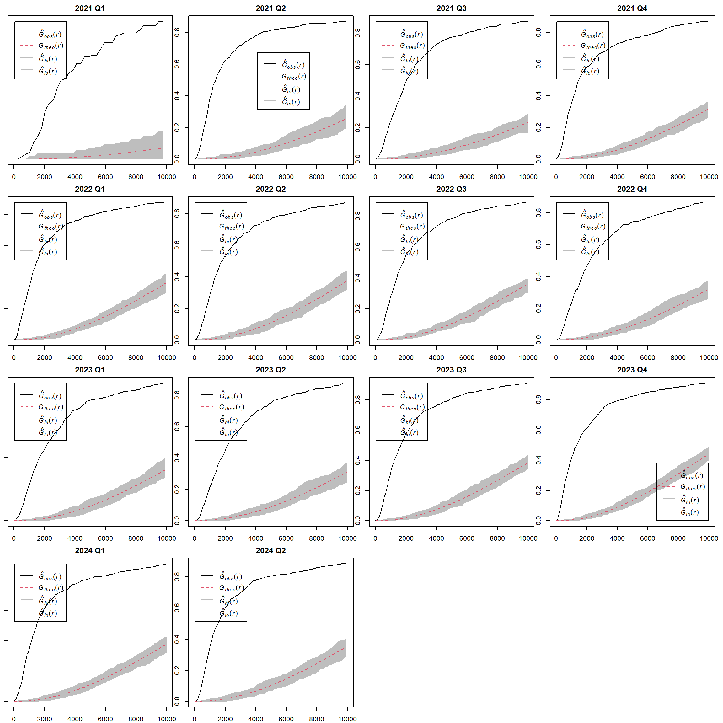
Violence against civilians overview
set.seed(126)

# Create a list of all the ER quarter datasets
er_datasets <- list(
  my_2021_Q1_VAC_quarter_data_regions_ppp,
  my_2021_Q2_VAC_quarter_data_regions_ppp,
  my_2021_Q3_VAC_quarter_data_regions_ppp,
  my_2021_Q4_VAC_quarter_data_regions_ppp,
  my_2022_Q1_VAC_quarter_data_regions_ppp,
  my_2022_Q2_VAC_quarter_data_regions_ppp,
  my_2022_Q3_VAC_quarter_data_regions_ppp,
  my_2022_Q4_VAC_quarter_data_regions_ppp,
  my_2023_Q1_VAC_quarter_data_regions_ppp,
  my_2023_Q2_VAC_quarter_data_regions_ppp,
  my_2023_Q3_VAC_quarter_data_regions_ppp,
  my_2023_Q4_VAC_quarter_data_regions_ppp,
  my_2024_Q1_VAC_quarter_data_regions_ppp,
  my_2024_Q2_VAC_quarter_data_regions_ppp
)

# Corresponding year and quarter labels for the plots
er_labels <- c(
  "2021 Q1", "2021 Q2", "2021 Q3", "2021 Q4",
  "2022 Q1", "2022 Q2", "2022 Q3", "2022 Q4",
  "2023 Q1", "2023 Q2", "2023 Q3", "2023 Q4",
  "2024 Q1", "2024 Q2"
)

# Set up the plotting area
par(mar = c(2,1,2,1))
par(mfrow=c(4,4))

# Loop through each dataset and create the KDE plots
for (i in seq_along(er_datasets)) {
    G_CK.csr <- envelope(er_datasets[[i]], Gest, nsim = 50, parallel = parallel::detectCores())
  plot(G_CK.csr, xlim=c(0,10000), main= er_labels[[i]])
}
Generating 50 simulations of CSR ...
1, 2, 3, 4, 5, 6, 7, 8, 9, 10, 11, 12, 13, 14, 15, 16, 17, 18, 19, 20,
21, 22, 23, 24, 25, 26, 27, 28, 29, 30, 31, 32, 33, 34, 35, 36, 37, 38, 39, 40,
41, 42, 43, 44, 45, 46, 47, 48, 49,
50.
Done.Generating 50 simulations of CSR ...
1, 2, 3, 4, 5, 6, 7, 8, 9, 10, 11, 12, 13, 14, 15, 16, 17, 18, 19, 20,
21, 22, 23, 24, 25, 26, 27, 28, 29, 30, 31, 32, 33, 34, 35, 36, 37, 38, 39, 40,
41, 42, 43, 44, 45, 46, 47, 48, 49,
50.
Done.Generating 50 simulations of CSR ...
1, 2, 3, 4, 5, 6, 7, 8, 9, 10, 11, 12, 13, 14, 15, 16, 17, 18, 19, 20,
21, 22, 23, 24, 25, 26, 27, 28, 29, 30, 31, 32, 33, 34, 35, 36, 37, 38, 39, 40,
41, 42, 43, 44, 45, 46, 47, 48, 49,
50.
Done.Generating 50 simulations of CSR ...
1, 2, 3, 4, 5, 6, 7, 8, 9, 10, 11, 12, 13, 14, 15, 16, 17, 18, 19, 20,
21, 22, 23, 24, 25, 26, 27, 28, 29, 30, 31, 32, 33, 34, 35, 36, 37, 38, 39, 40,
41, 42, 43, 44, 45, 46, 47, 48, 49,
50.
Done.Generating 50 simulations of CSR ...
1, 2, 3, 4, 5, 6, 7, 8, 9, 10, 11, 12, 13, 14, 15, 16, 17, 18, 19, 20,
21, 22, 23, 24, 25, 26, 27, 28, 29, 30, 31, 32, 33, 34, 35, 36, 37, 38, 39, 40,
41, 42, 43, 44, 45, 46, 47, 48, 49,
50.
Done.Generating 50 simulations of CSR ...
1, 2, 3, 4, 5, 6, 7, 8, 9, 10, 11, 12, 13, 14, 15, 16, 17, 18, 19, 20,
21, 22, 23, 24, 25, 26, 27, 28, 29, 30, 31, 32, 33, 34, 35, 36, 37, 38, 39, 40,
41, 42, 43, 44, 45, 46, 47, 48, 49,
50.
Done.Generating 50 simulations of CSR ...
1, 2, 3, 4, 5, 6, 7, 8, 9, 10, 11, 12, 13, 14, 15, 16, 17, 18, 19, 20,
21, 22, 23, 24, 25, 26, 27, 28, 29, 30, 31, 32, 33, 34, 35, 36, 37, 38, 39, 40,
41, 42, 43, 44, 45, 46, 47, 48, 49,
50.
Done.Generating 50 simulations of CSR ...
1, 2, 3, 4, 5, 6, 7, 8, 9, 10, 11, 12, 13, 14, 15, 16, 17, 18, 19, 20,
21, 22, 23, 24, 25, 26, 27, 28, 29, 30, 31, 32, 33, 34, 35, 36, 37, 38, 39, 40,
41, 42, 43, 44, 45, 46, 47, 48, 49,
50.
Done.Generating 50 simulations of CSR ...
1, 2, 3, 4, 5, 6, 7, 8, 9, 10, 11, 12, 13, 14, 15, 16, 17, 18, 19, 20,
21, 22, 23, 24, 25, 26, 27, 28, 29, 30, 31, 32, 33, 34, 35, 36, 37, 38, 39, 40,
41, 42, 43, 44, 45, 46, 47, 48, 49,
50.
Done.Generating 50 simulations of CSR ...
1, 2, 3, 4, 5, 6, 7, 8, 9, 10, 11, 12, 13, 14, 15, 16, 17, 18, 19, 20,
21, 22, 23, 24, 25, 26, 27, 28, 29, 30, 31, 32, 33, 34, 35, 36, 37, 38, 39, 40,
41, 42, 43, 44, 45, 46, 47, 48, 49,
50.
Done.Generating 50 simulations of CSR ...
1, 2, 3, 4, 5, 6, 7, 8, 9, 10, 11, 12, 13, 14, 15, 16, 17, 18, 19, 20,
21, 22, 23, 24, 25, 26, 27, 28, 29, 30, 31, 32, 33, 34, 35, 36, 37, 38, 39, 40,
41, 42, 43, 44, 45, 46, 47, 48, 49,
50.
Done.Generating 50 simulations of CSR ...
1, 2, 3, 4, 5, 6, 7, 8, 9, 10, 11, 12, 13, 14, 15, 16, 17, 18, 19, 20,
21, 22, 23, 24, 25, 26, 27, 28, 29, 30, 31, 32, 33, 34, 35, 36, 37, 38, 39, 40,
41, 42, 43, 44, 45, 46, 47, 48, 49,
50.
Done.Generating 50 simulations of CSR ...
1, 2, 3, 4, 5, 6, 7, 8, 9, 10, 11, 12, 13, 14, 15, 16, 17, 18, 19, 20,
21, 22, 23, 24, 25, 26, 27, 28, 29, 30, 31, 32, 33, 34, 35, 36, 37, 38, 39, 40,
41, 42, 43, 44, 45, 46, 47, 48, 49,
50.
Done.Generating 50 simulations of CSR ...
1, 2, 3, 4, 5, 6, 7, 8, 9, 10, 11, 12, 13, 14, 15, 16, 17, 18, 19, 20,
21, 22, 23, 24, 25, 26, 27, 28, 29, 30, 31, 32, 33, 34, 35, 36, 37, 38, 39, 40,
41, 42, 43, 44, 45, 46, 47, 48, 49,
50.
Done.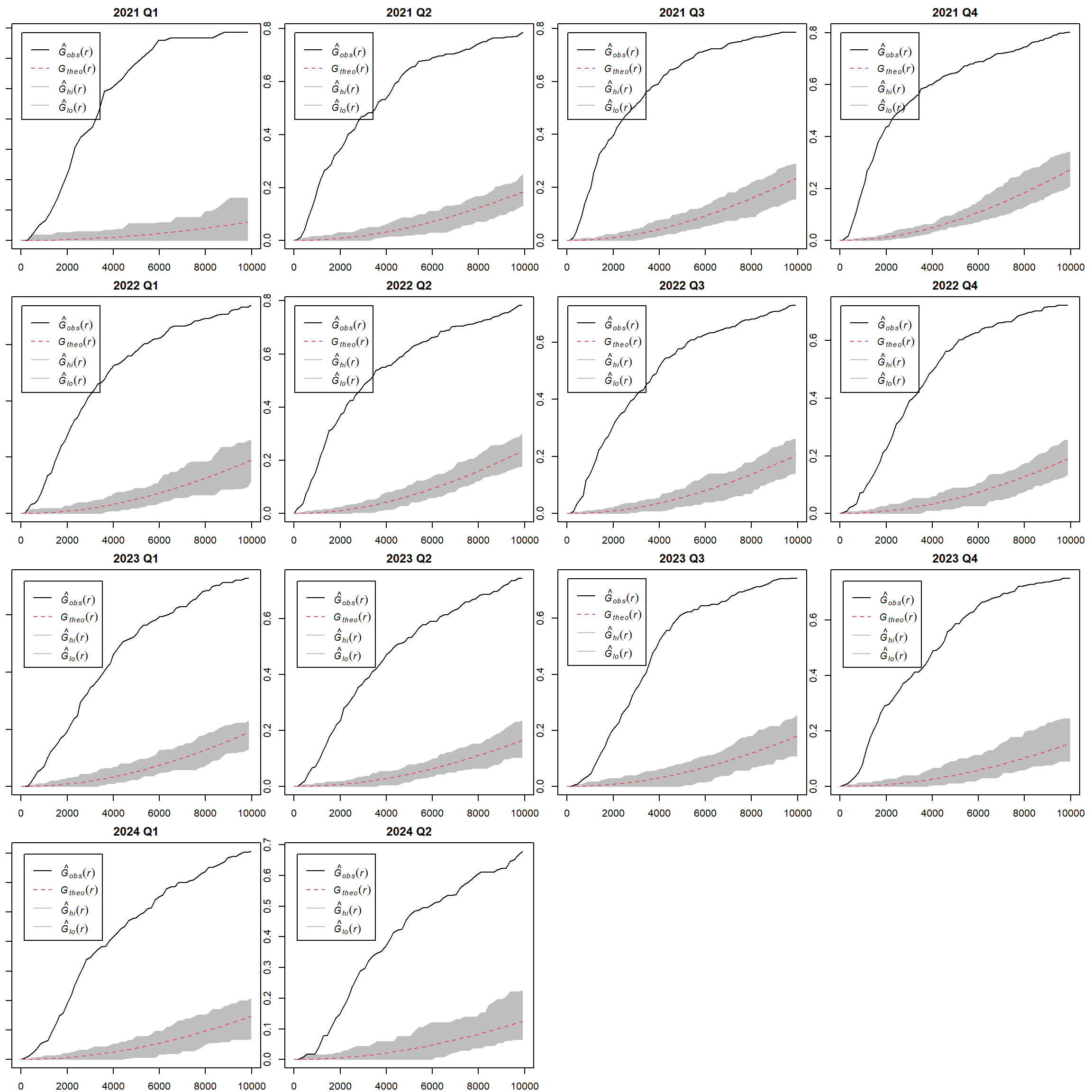
Note
Quarter-wise analysis for all event types:
2021 Q1: There is a strong deviation from the CSR, where the empirical G-function lies well above the envelope. This suggests clustering, particularly over the distances considered.
2021 Q2 to 2024 Q2: Most quarters show a more stable pattern with the empirical G-function generally falling within the simulation envelope or only slightly above it at different distances. This suggests that there is no significant deviation from CSR, implying randomness in the spatial arrangement of points during most of these quarters. In some cases, the curve slightly rises above the envelope, which could indicate mild clustering.
General Trend: Across the quarters, the empirical G-function mostly lies within the CSR envelope, indicating a spatial point pattern that does not strongly deviate from randomness. The early quarters show more clustering, but later quarters become more consistent with random spatial distribution.
1.7 Determining Spatio-Temporal KDE Layer
1.7.1 Visualising geographic distribution of events by month
We would first prepare the acled_sf object. The q column is derived from the event_date field using the quarter() function, which extracts the quarter (Q1, Q2, Q3, or Q4) from each date. This new column helps in grouping events by the quarter of the year, which is crucial for spatio-temporal analysis.
temporal_acled_sf <- acled_sf %>%
mutate(q = quarter(event_date))
write_rds(temporal_acled_sf, "data/rds/temporal_acled_sf.rds")tm_shape(regions_sf)+
tm_polygons() +
tm_shape(temporal_acled_sf) +
tm_dots() +
tm_facets(by="quarter",
free.coords=FALSE,
drop.units = TRUE)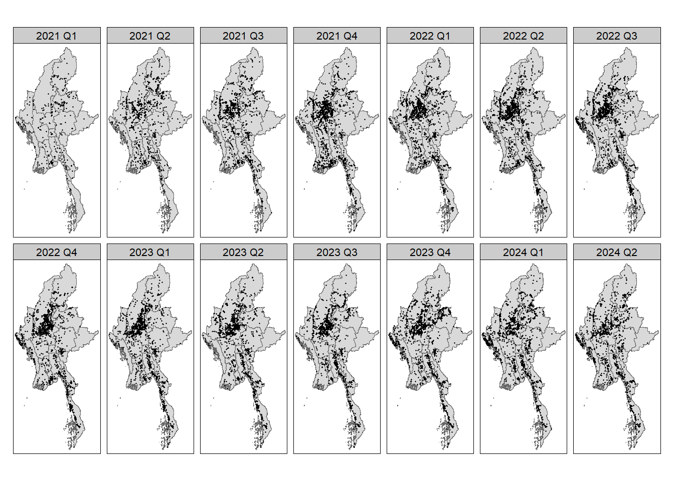
1.7.2 Deriving Quarterly Spatio-Temporal KDE Layers
In this section, we will be generating Quarterly Spatio-Temporal KDE (Kernel Density Estimation) layers for conflict events. KDE is a powerful technique for estimating the probability density function of a random variable—in this case, spatial point events such as conflicts.
The goal of spatio-temporal KDE is to analyze how the intensity of conflict events evolves both spatially and temporally. Instead of simply plotting the points, KDE smooths the data to show areas of higher and lower event intensity, giving a more nuanced view of conflict pattern
::: Key Steps in this Section: 1. Quarter-Based Data Aggregation: The conflict data will be divided into quarters (e.g., Q1 to Q4), allowing us to analyze conflict intensity in each three-month period.
Spatial Density Calculation: The KDE method will be applied to the spatial points in each quarter, resulting in a density surface that highlights areas of high conflict concentration. This is more informative than a simple point map, as it reveals underlying patterns that might not be obvious from the raw data.
Temporal Change Analysis: By deriving KDE layers for each quarter, you will visualize how conflict intensity shifts over time. This allows you to examine whether certain regions experience persistent conflict or if the hotspots move across the country as the year progresses.
Visualizing KDE Layers: Each KDE layer will be visualized on a map, either as a standalone plot or as part of a sequence (e.g., an animated GIF), showing how the density changes quarterly. This provides a dynamic view of the conflict landscape.
:::
1.7.2.1 Explosions/Remote violence
Example <- "Explosions/Remote violence"
acled_quarters_2021_ppp <- as.ppp(temporal_acled_sf %>%
filter(year == 2021 & event_type == Example) %>%
select(q))
acled_quarters_2022_ppp <- as.ppp(temporal_acled_sf %>%
filter(year == 2022 & event_type == Example) %>%
select(q))
acled_quarters_2023_ppp <- as.ppp(temporal_acled_sf %>%
filter(year == 2023 & event_type == Example) %>%
select(q))
acled_quarters_2024_ppp <- as.ppp(temporal_acled_sf %>%
filter(year == 2024 & event_type == Example) %>%
select(q))acled_spatio_ppp_owin <- acled_quarters_2021_ppp[regions_owin]
st_kde <- spattemp.density(acled_spatio_ppp_owin)
tims <- c(1, 3, 2, 4)
par(mfcol=c(2,2))
for(i in tims){
plot(st_kde, i,
override.par=FALSE,
fix.range=TRUE,
main=paste("KDE at 2021 Q",i))
}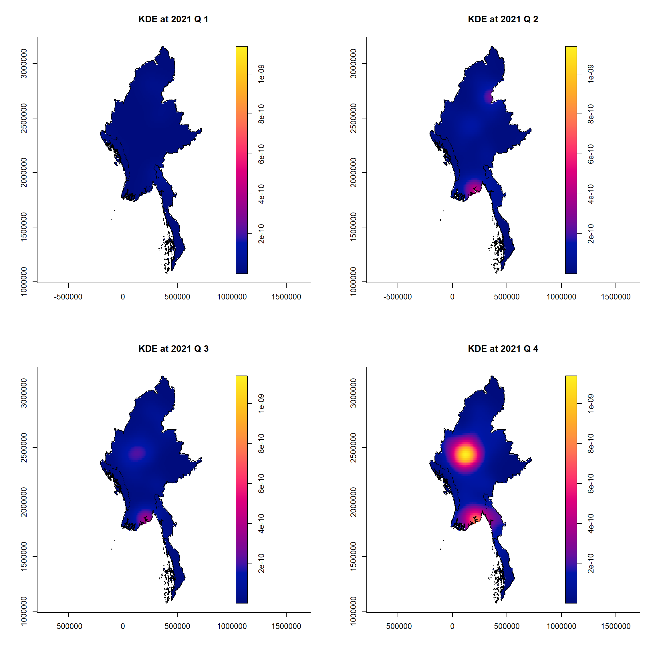
for(i in tims){
png(filename = paste0("data/rds/kde_plots/ER/kde_2021_ER", i, ".png"), width = 800, height = 600)
plot(st_kde, i,
override.par=FALSE,
fix.range=TRUE,
main=paste("KDE at 2021 Q",i))
dev.off()
}acled_spatio_ppp_owin <- acled_quarters_2022_ppp[regions_owin]
st_kde <- spattemp.density(acled_spatio_ppp_owin)
tims <- c(1, 3, 2, 4)
par(mfcol=c(2,2))
for(i in tims){
plot(st_kde, i,
override.par=FALSE,
fix.range=TRUE,
main=paste("KDE at 2022 Q",i))
}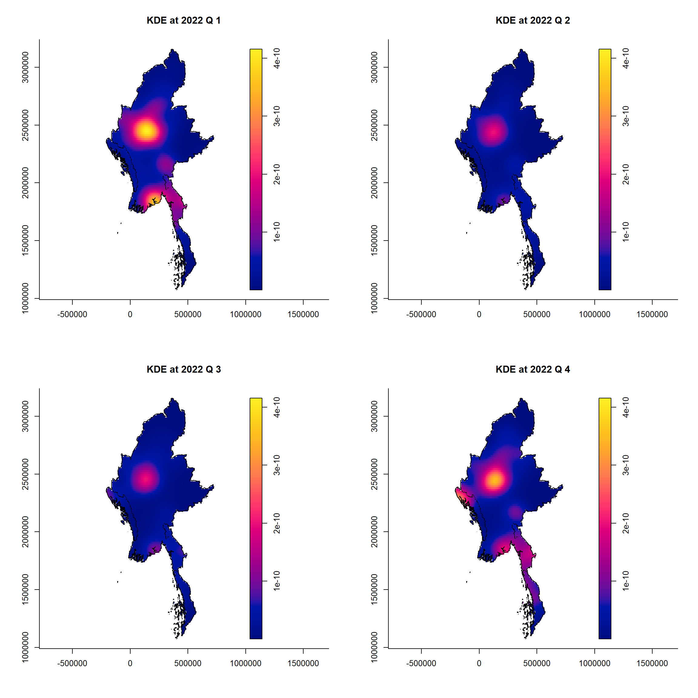
for(i in tims){
png(filename = paste0("data/rds/kde_plots/ER/kde_2022_ER", i, ".png"), width = 800, height = 600)
plot(st_kde, i,
override.par=FALSE,
fix.range=TRUE,
main=paste("KDE at 2022 Q",i))
dev.off()
}acled_spatio_ppp_owin <- acled_quarters_2023_ppp[regions_owin]
st_kde <- spattemp.density(acled_spatio_ppp_owin)
tims <- c(1, 3, 2, 4)
par(mfcol=c(2,2))
for(i in tims){
plot(st_kde, i,
override.par=FALSE,
fix.range=TRUE,
main=paste("KDE at 2023 Q",i))
}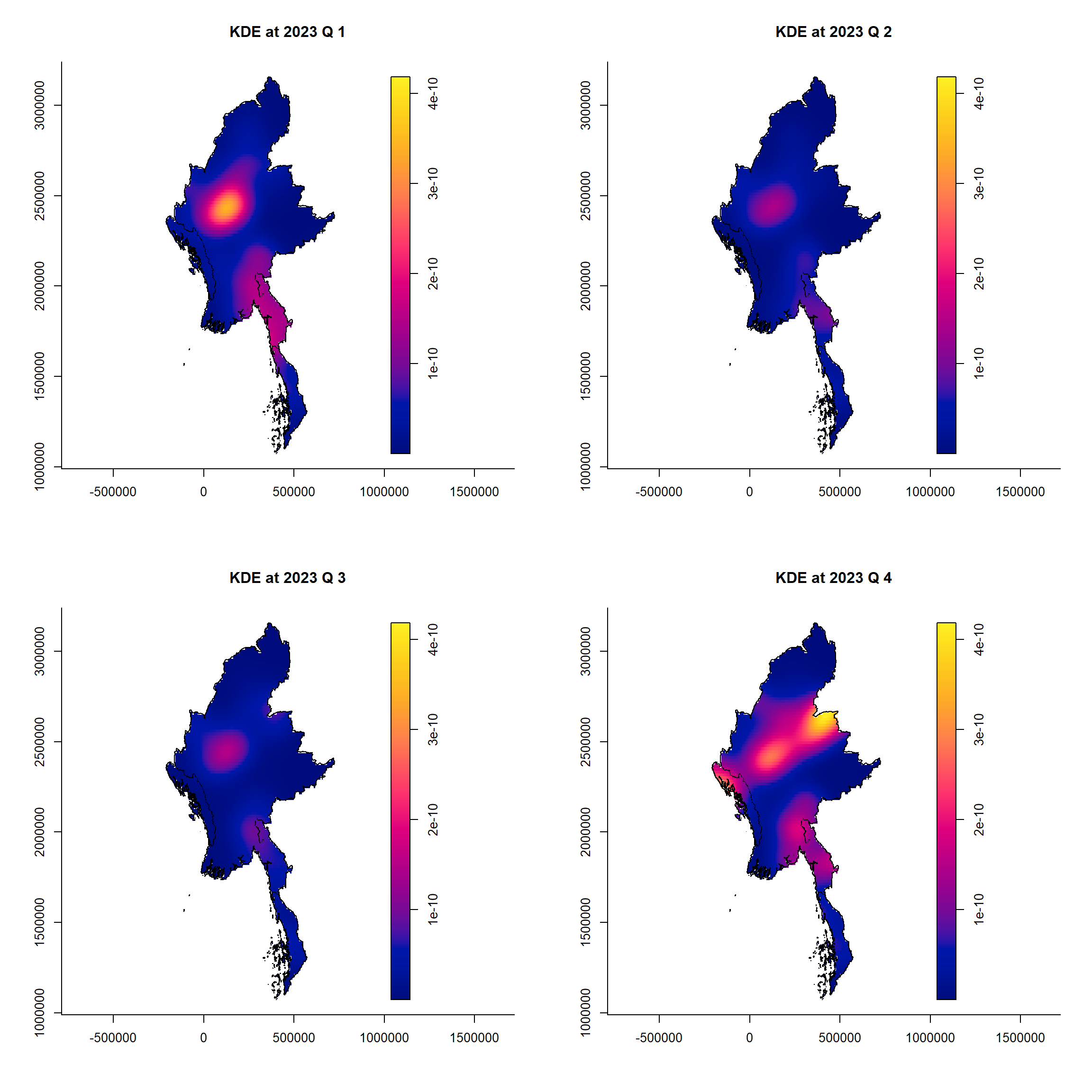
for(i in tims){
png(filename = paste0("data/rds/kde_plots/ER/kde_2023_ER", i, ".png"), width = 800, height = 600)
plot(st_kde, i,
override.par=FALSE,
fix.range=TRUE,
main=paste("KDE at 2023 Q",i))
dev.off()
}acled_spatio_ppp_owin <- acled_quarters_2024_ppp[regions_owin]
st_kde <- spattemp.density(acled_spatio_ppp_owin)
tims <- c(1, 2)
par(mfrow=c(1,2))
for(i in tims){
plot(st_kde, i,
override.par=FALSE,
fix.range=TRUE,
main=paste("KDE at 2024 Q",i))
}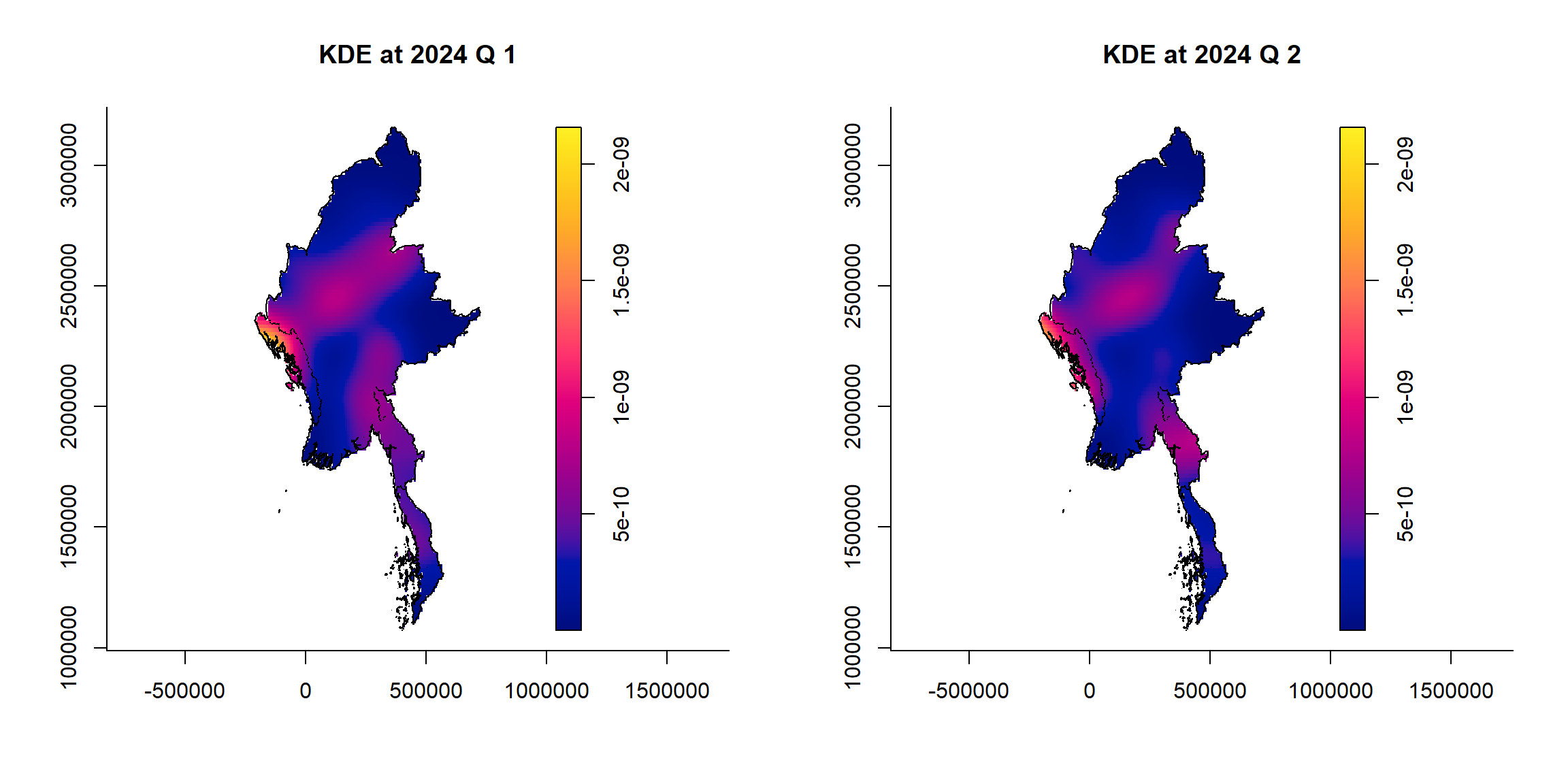
for(i in tims){
png(filename = paste0("data/rds/kde_plots/ER/kde_2024_ER", i, ".png"), width = 800, height = 600)
plot(st_kde, i,
override.par=FALSE,
fix.range=TRUE,
main=paste("KDE at 2024 Q",i))
dev.off()
}kde_images <- list.files("data/rds/kde_plots/ER/", full.names = TRUE, pattern = ".png")
image_read(kde_images) %>%
image_animate(fps = 2)
1.7.2.2 Strategic developments
Example <- "Strategic developments"
acled_quarters_2021_ppp <- as.ppp(temporal_acled_sf %>%
filter(year == 2021 & event_type == Example) %>%
select(q))
acled_quarters_2022_ppp <- as.ppp(temporal_acled_sf %>%
filter(year == 2022 & event_type == Example) %>%
select(q))
acled_quarters_2023_ppp <- as.ppp(temporal_acled_sf %>%
filter(year == 2023 & event_type == Example) %>%
select(q))
acled_quarters_2024_ppp <- as.ppp(temporal_acled_sf %>%
filter(year == 2024 & event_type == Example) %>%
select(q))acled_spatio_ppp_owin <- acled_quarters_2021_ppp[regions_owin]
st_kde <- spattemp.density(acled_spatio_ppp_owin)
tims <- c(1, 3, 2, 4)
par(mfcol=c(2,2))
for(i in tims){
plot(st_kde, i,
override.par=FALSE,
fix.range=TRUE,
main=paste("KDE at 2021 Q",i))
}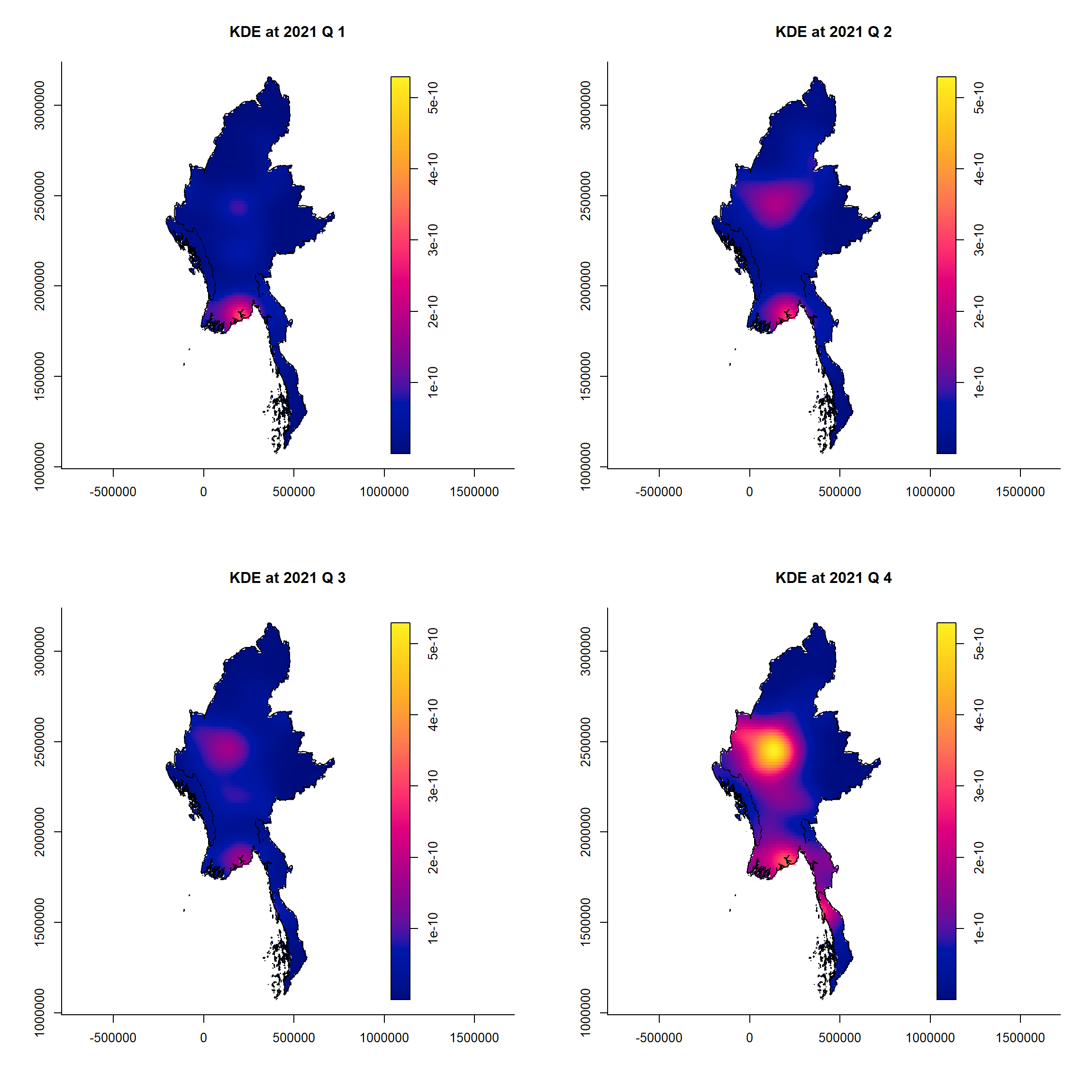
for(i in tims){
png(filename = paste0("data/rds/kde_plots/SD/kde_2021_SD", i, ".png"), width = 800, height = 600)
plot(st_kde, i,
override.par=FALSE,
fix.range=TRUE,
main=paste("KDE at 2021 Q",i))
dev.off()
}acled_spatio_ppp_owin <- acled_quarters_2022_ppp[regions_owin]
st_kde <- spattemp.density(acled_spatio_ppp_owin)
tims <- c(1, 3, 2, 4)
par(mfcol=c(2,2))
for(i in tims){
plot(st_kde, i,
override.par=FALSE,
fix.range=TRUE,
main=paste("KDE at 2022 Q",i))
}
for(i in tims){
png(filename = paste0("data/rds/kde_plots/SD/kde_2022_SD", i, ".png"), width = 800, height = 600)
plot(st_kde, i,
override.par=FALSE,
fix.range=TRUE,
main=paste("KDE at 2022 Q",i))
dev.off()
}acled_spatio_ppp_owin <- acled_quarters_2023_ppp[regions_owin]
st_kde <- spattemp.density(acled_spatio_ppp_owin)
tims <- c(1, 3, 2, 4)
par(mfcol=c(2,2))
for(i in tims){
plot(st_kde, i,
override.par=FALSE,
fix.range=TRUE,
main=paste("KDE at 2023 Q",i))
}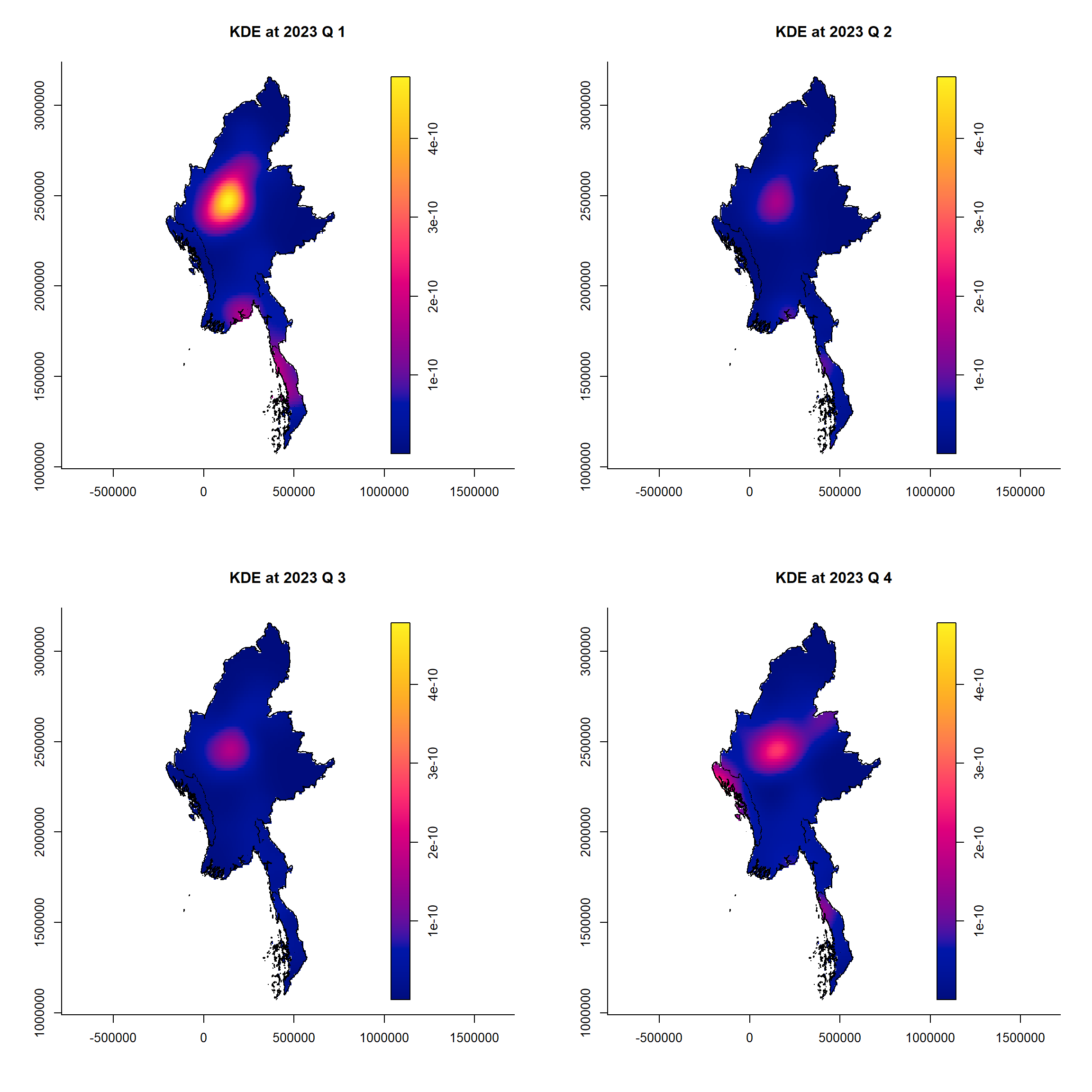
for(i in tims){
png(filename = paste0("data/rds/kde_plots/SD/kde_2023_SD", i, ".png"), width = 800, height = 600)
plot(st_kde, i,
override.par=FALSE,
fix.range=TRUE,
main=paste("KDE at 2023 Q",i))
dev.off()
}acled_spatio_ppp_owin <- acled_quarters_2024_ppp[regions_owin]
st_kde <- spattemp.density(acled_spatio_ppp_owin)
tims <- c(1, 2)
par(mfrow=c(1,2))
for(i in tims){
plot(st_kde, i,
override.par=FALSE,
fix.range=TRUE,
main=paste("KDE at 2024 Q",i))
}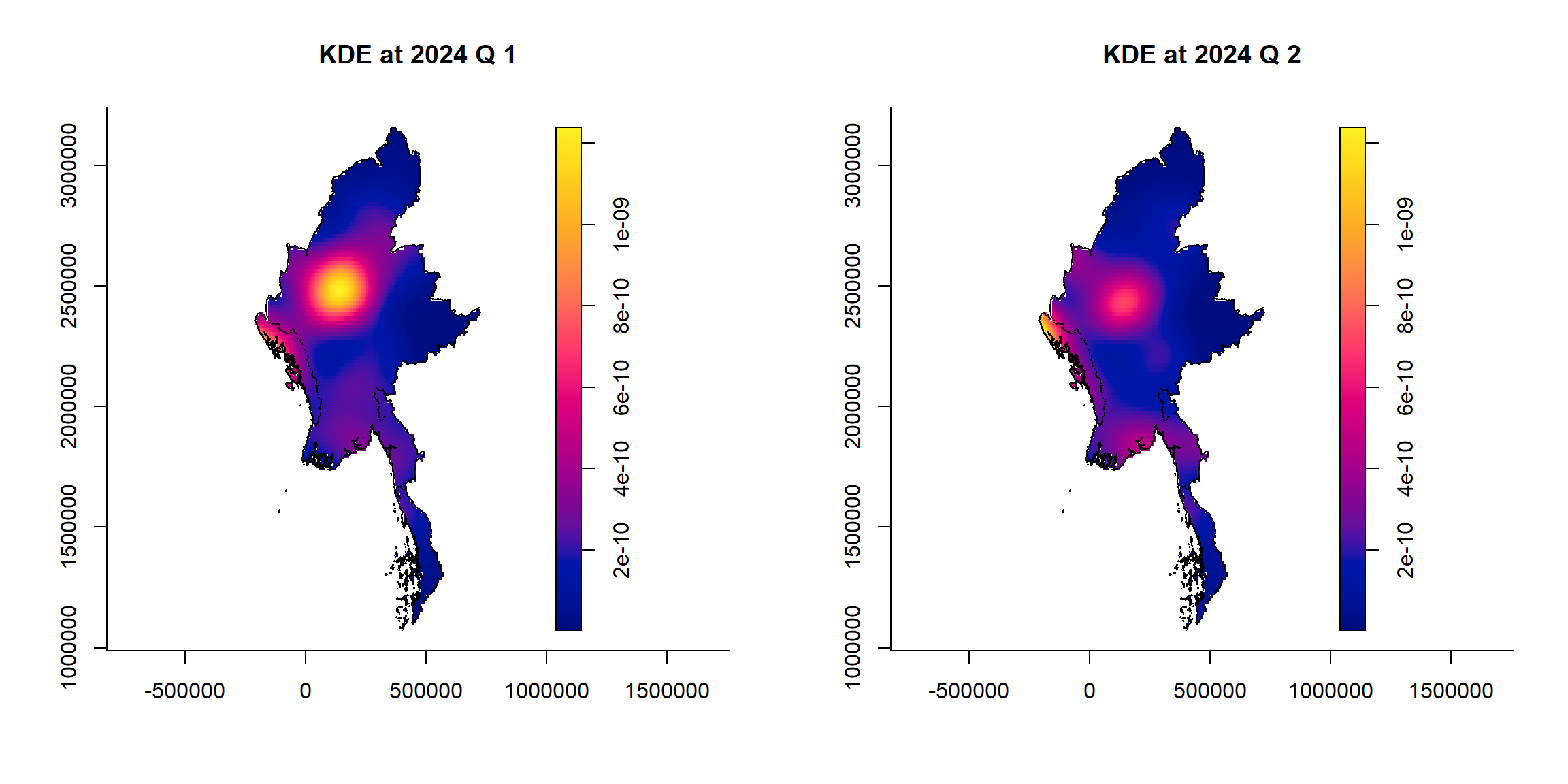
for(i in tims){
png(filename = paste0("data/rds/kde_plots/SD/kde_2024_SD", i, ".png"), width = 800, height = 600)
plot(st_kde, i,
override.par=FALSE,
fix.range=TRUE,
main=paste("KDE at 2024 Q",i))
dev.off()
}kde_images <- list.files("data/rds/kde_plots/SD/", full.names = TRUE, pattern = ".png")
image_read(kde_images) %>%
image_animate(fps = 2)
1.7.2.3 Battles
Example <- "Battles"
acled_quarters_2021_ppp <- as.ppp(temporal_acled_sf %>%
filter(year == 2021 & event_type == Example) %>%
select(q))
acled_quarters_2022_ppp <- as.ppp(temporal_acled_sf %>%
filter(year == 2022 & event_type == Example) %>%
select(q))
acled_quarters_2023_ppp <- as.ppp(temporal_acled_sf %>%
filter(year == 2023 & event_type == Example) %>%
select(q))
acled_quarters_2024_ppp <- as.ppp(temporal_acled_sf %>%
filter(year == 2024 & event_type == Example) %>%
select(q))acled_spatio_ppp_owin <- acled_quarters_2021_ppp[regions_owin]
st_kde <- spattemp.density(acled_spatio_ppp_owin)
tims <- c(1, 3, 2, 4)
par(mfcol=c(2,2))
for(i in tims){
plot(st_kde, i,
override.par=FALSE,
fix.range=TRUE,
main=paste("KDE at 2021 Q",i))
}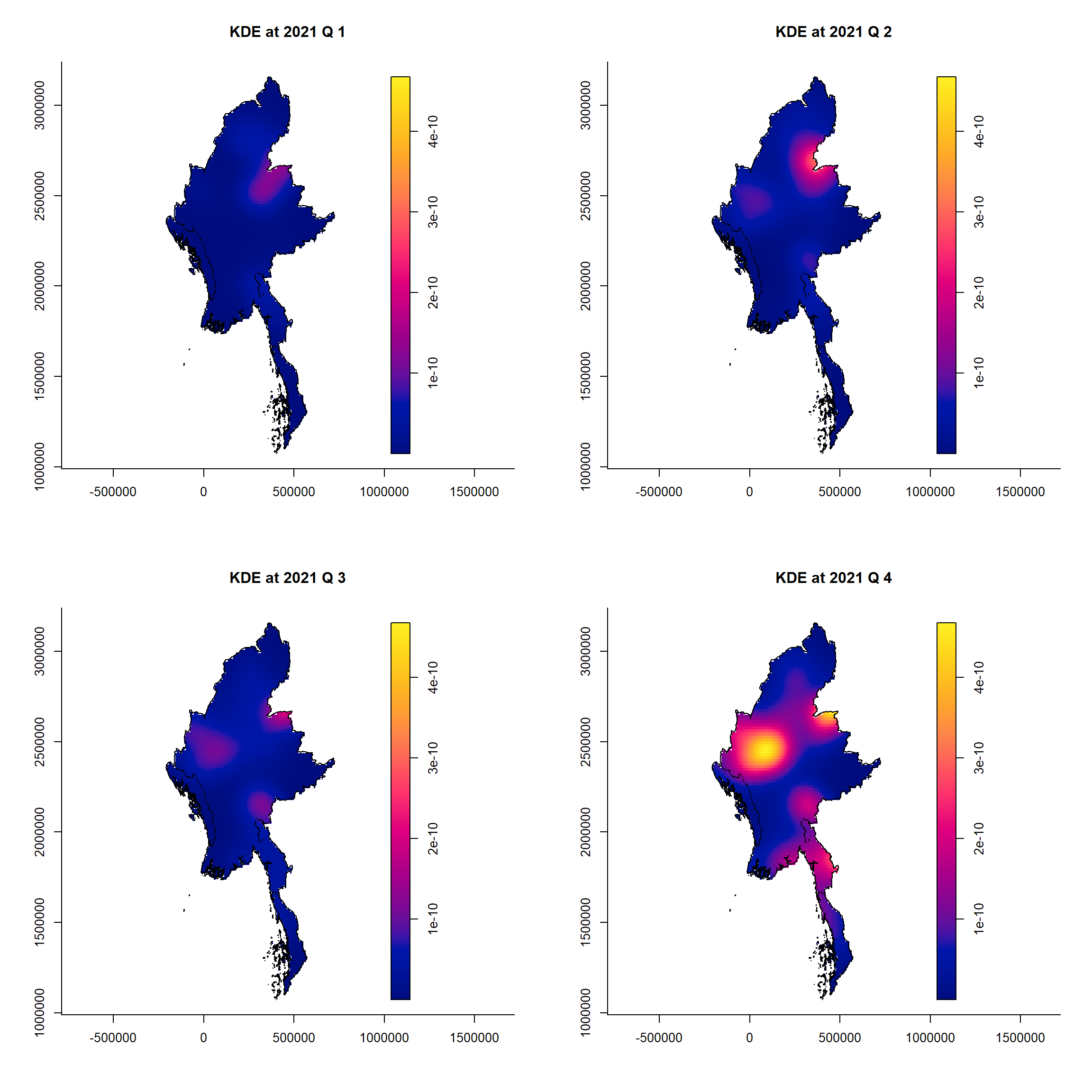
for(i in tims){
png(filename = paste0("data/rds/kde_plots/B/kde_2021_B", i, ".png"), width = 800, height = 600)
plot(st_kde, i,
override.par=FALSE,
fix.range=TRUE,
main=paste("KDE at 2021 Q",i))
dev.off()
}acled_spatio_ppp_owin <- acled_quarters_2022_ppp[regions_owin]
st_kde <- spattemp.density(acled_spatio_ppp_owin)
tims <- c(1, 3, 2, 4)
par(mfcol=c(2,2))
for(i in tims){
plot(st_kde, i,
override.par=FALSE,
fix.range=TRUE,
main=paste("KDE at 2022 Q",i))
}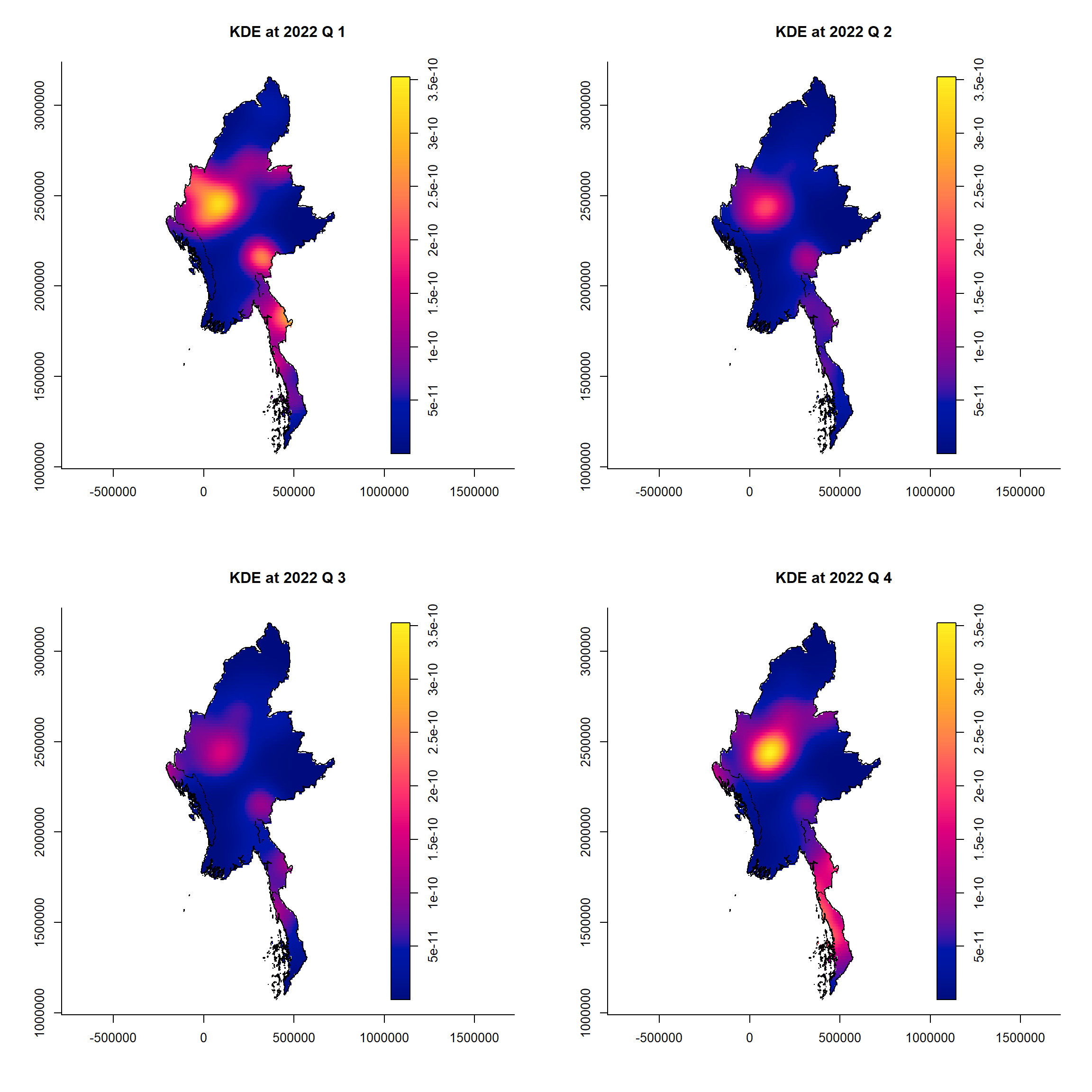
for(i in tims){
png(filename = paste0("data/rds/kde_plots/B/kde_2022_B", i, ".png"), width = 800, height = 600)
plot(st_kde, i,
override.par=FALSE,
fix.range=TRUE,
main=paste("KDE at 2022 Q",i))
dev.off()
}acled_spatio_ppp_owin <- acled_quarters_2023_ppp[regions_owin]
st_kde <- spattemp.density(acled_spatio_ppp_owin)
tims <- c(1, 3, 2, 4)
par(mfcol=c(2,2))
for(i in tims){
plot(st_kde, i,
override.par=FALSE,
fix.range=TRUE,
main=paste("KDE at 2023 Q",i))
}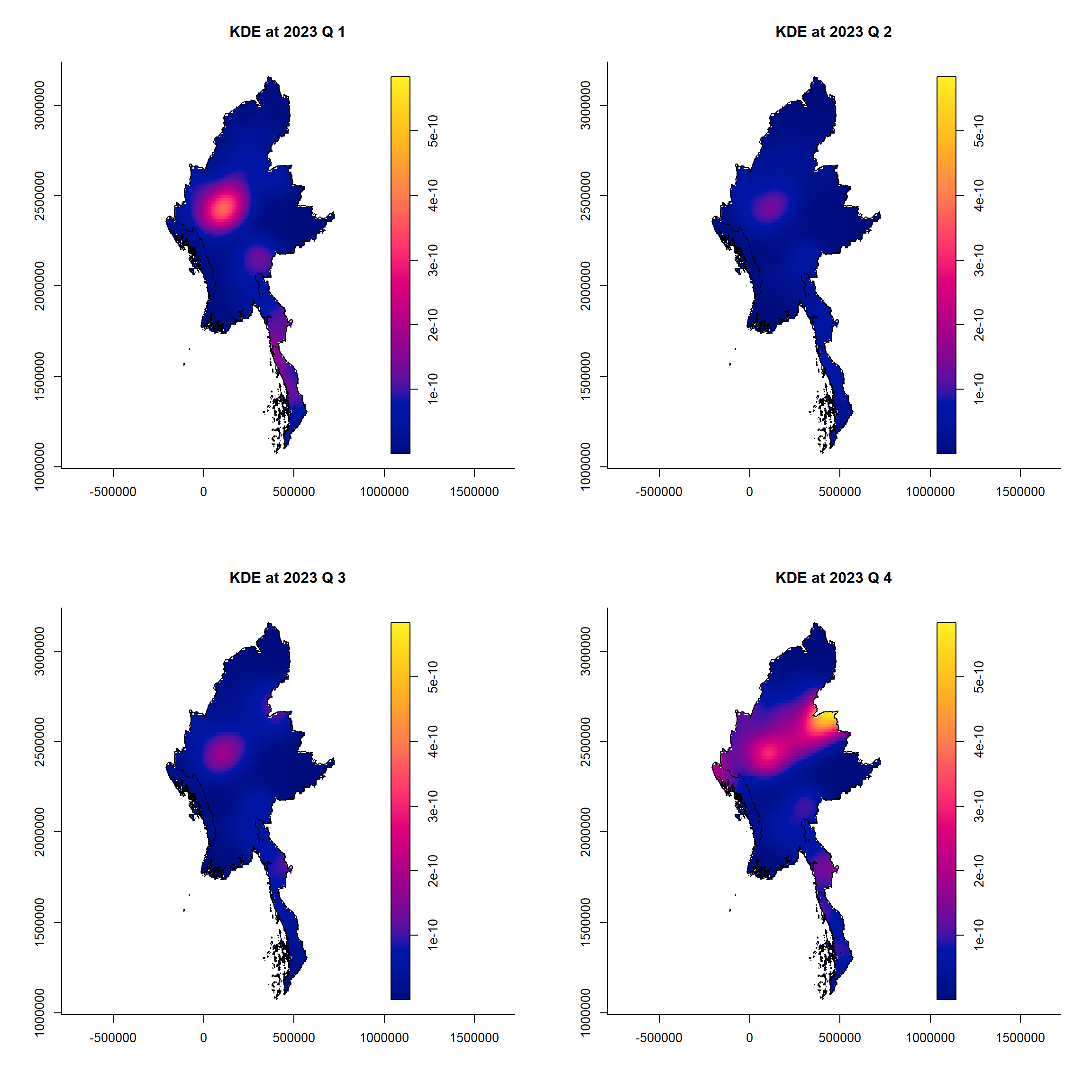
for(i in tims){
png(filename = paste0("data/rds/kde_plots/B/kde_2023_B", i, ".png"), width = 800, height = 600)
plot(st_kde, i,
override.par=FALSE,
fix.range=TRUE,
main=paste("KDE at 2023 Q",i))
dev.off()
}acled_spatio_ppp_owin <- acled_quarters_2024_ppp[regions_owin]
st_kde <- spattemp.density(acled_spatio_ppp_owin)
tims <- c(1, 2)
par(mfrow=c(1,2))
for(i in tims){
plot(st_kde, i,
override.par=FALSE,
fix.range=TRUE,
main=paste("KDE at 2024 Q",i))
}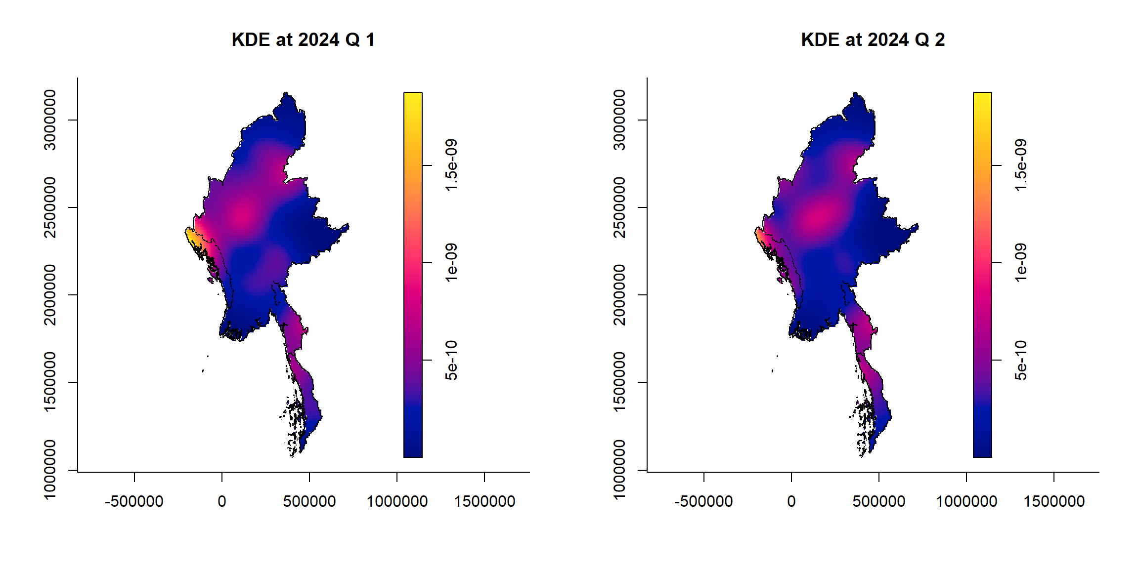
for(i in tims){
png(filename = paste0("data/rds/kde_plots/B/kde_2024_B", i, ".png"), width = 800, height = 600)
plot(st_kde, i,
override.par=FALSE,
fix.range=TRUE,
main=paste("KDE at 2024 Q",i))
dev.off()
}kde_images <- list.files("data/rds/kde_plots/B/", full.names = TRUE, pattern = ".png")
image_read(kde_images) %>%
image_animate(fps = 2)
1.7.2.4 Violence against civilians
Example <- "Violence against civilians"
acled_quarters_2021_ppp <- as.ppp(temporal_acled_sf %>%
filter(year == 2021 & event_type == Example) %>%
select(q))
acled_quarters_2022_ppp <- as.ppp(temporal_acled_sf %>%
filter(year == 2022 & event_type == Example) %>%
select(q))
acled_quarters_2023_ppp <- as.ppp(temporal_acled_sf %>%
filter(year == 2023 & event_type == Example) %>%
select(q))
acled_quarters_2024_ppp <- as.ppp(temporal_acled_sf %>%
filter(year == 2024 & event_type == Example) %>%
select(q))acled_spatio_ppp_owin <- acled_quarters_2021_ppp[regions_owin]
st_kde <- spattemp.density(acled_spatio_ppp_owin)
tims <- c(1, 3, 2, 4)
par(mfcol=c(2,2))
for(i in tims){
plot(st_kde, i,
override.par=FALSE,
fix.range=TRUE,
main=paste("KDE at 2021 Q",i))
}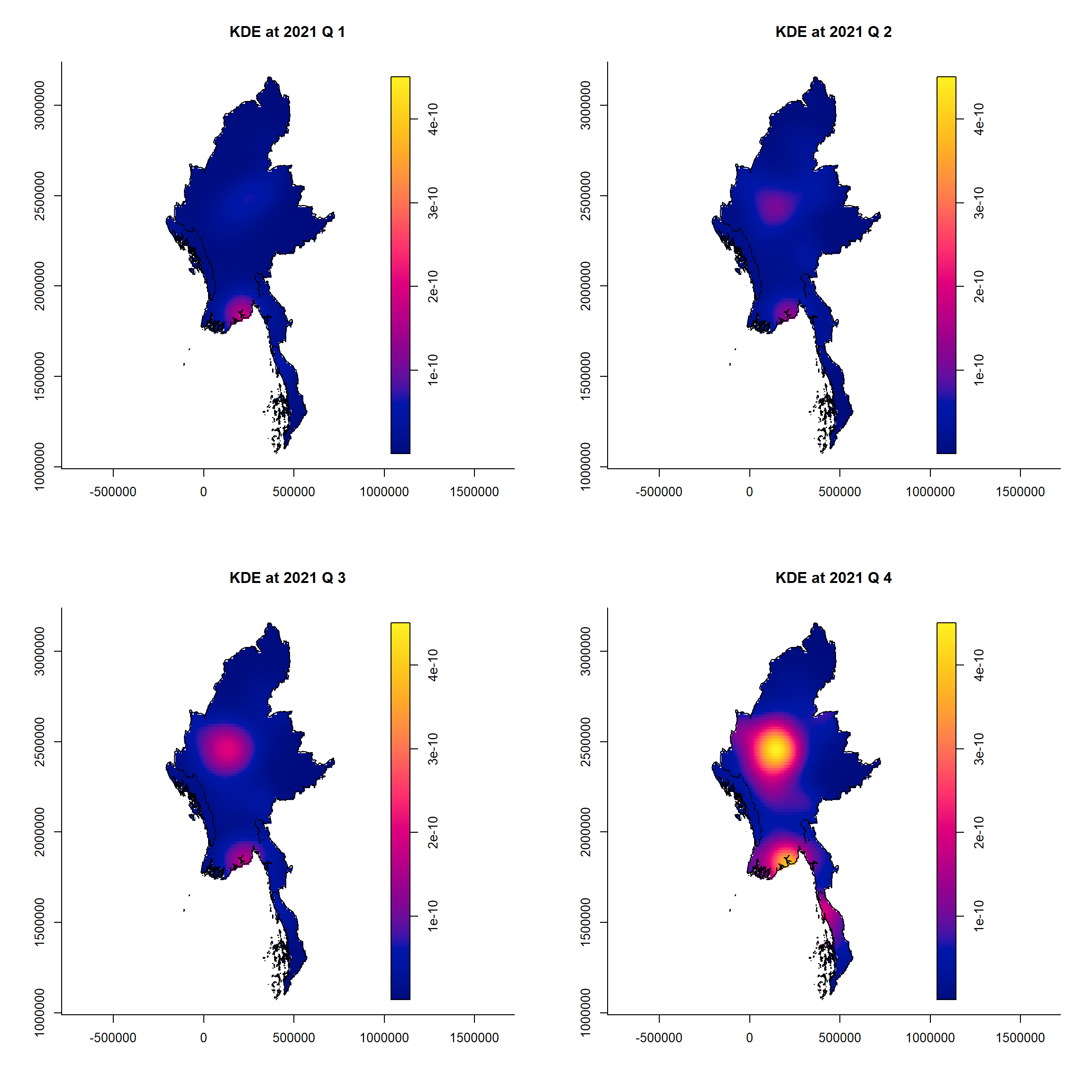
for(i in tims){
png(filename = paste0("data/rds/kde_plots/VAC/kde_2021_VAC", i, ".png"), width = 800, height = 600)
plot(st_kde, i,
override.par=FALSE,
fix.range=TRUE,
main=paste("KDE at 2021 Q",i))
dev.off()
}acled_spatio_ppp_owin <- acled_quarters_2022_ppp[regions_owin]
st_kde <- spattemp.density(acled_spatio_ppp_owin)
tims <- c(1, 3, 2, 4)
par(mfcol=c(2,2))
for(i in tims){
plot(st_kde, i,
override.par=FALSE,
fix.range=TRUE,
main=paste("KDE at 2022 Q",i))
}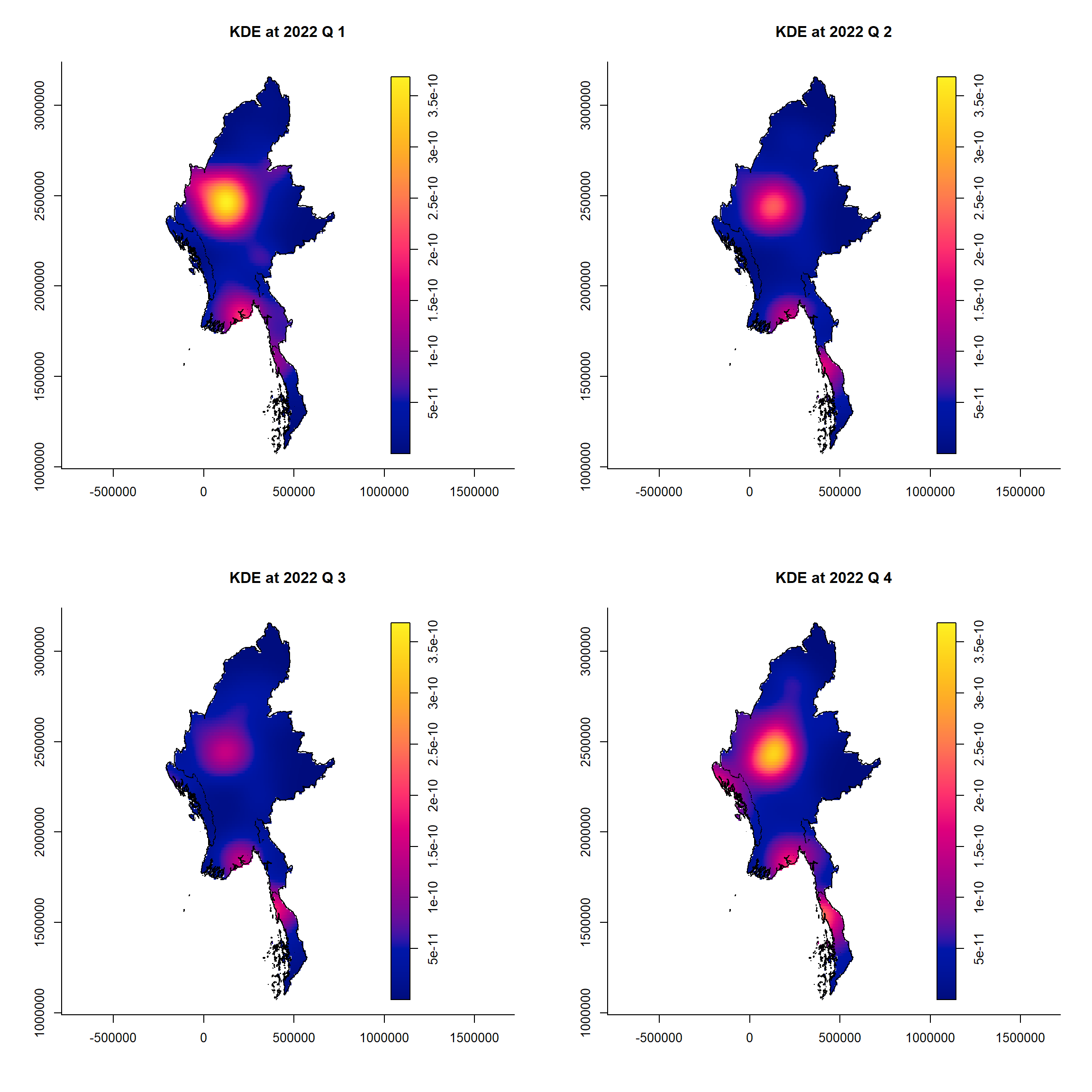
for(i in tims){
png(filename = paste0("data/rds/kde_plots/VAC/kde_2022_VAC", i, ".png"), width = 800, height = 600)
plot(st_kde, i,
override.par=FALSE,
fix.range=TRUE,
main=paste("KDE at 2022 Q",i))
dev.off()
}acled_spatio_ppp_owin <- acled_quarters_2023_ppp[regions_owin]
st_kde <- spattemp.density(acled_spatio_ppp_owin)
tims <- c(1, 3, 2, 4)
par(mfcol=c(2,2))
for(i in tims){
plot(st_kde, i,
override.par=FALSE,
fix.range=TRUE,
main=paste("KDE at 2023 Q",i))
}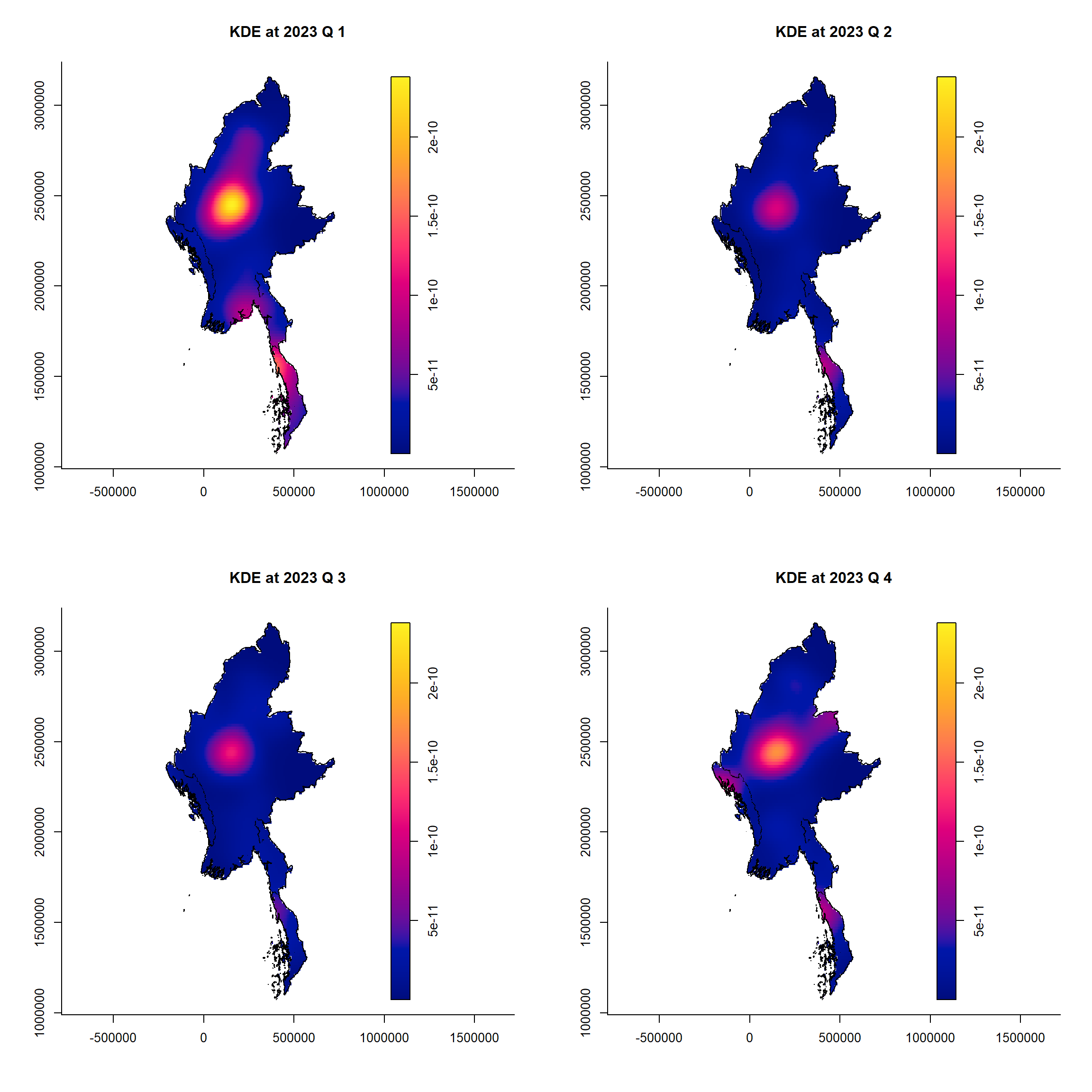
for(i in tims){
png(filename = paste0("data/rds/kde_plots/VAC/kde_2023_VAC", i, ".png"), width = 800, height = 600)
plot(st_kde, i,
override.par=FALSE,
fix.range=TRUE,
main=paste("KDE at 2023 Q",i))
dev.off()
}acled_spatio_ppp_owin <- acled_quarters_2024_ppp[regions_owin]
st_kde <- spattemp.density(acled_spatio_ppp_owin)
tims <- c(1, 2)
par(mfrow=c(1,2))
for(i in tims){
plot(st_kde, i,
override.par=FALSE,
fix.range=TRUE,
main=paste("KDE at 2024 Q",i))
}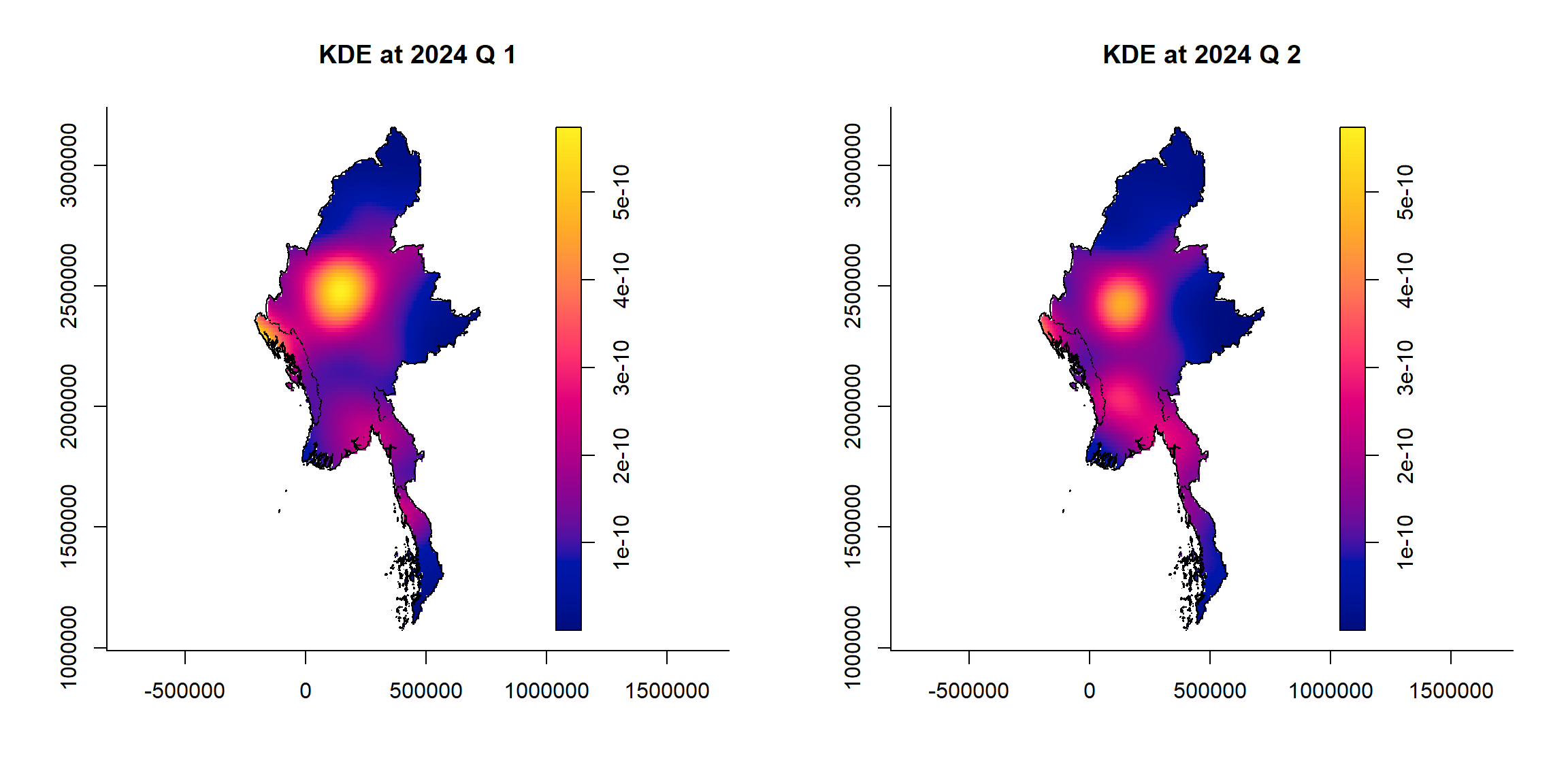
for(i in tims){
png(filename = paste0("data/rds/kde_plots/VAC/kde_2024_VAC", i, ".png"), width = 800, height = 600)
plot(st_kde, i,
override.par=FALSE,
fix.range=TRUE,
main=paste("KDE at 2024 Q",i))
dev.off()
}kde_images <- list.files("data/rds/kde_plots/VAC/", full.names = TRUE, pattern = ".png")
image_read(kde_images) %>%
image_animate(fps = 2)
1.8 2nd-Order Spatio-Temporal Point Patterns Analysis
Given that we are analyzing armed conflict data across different quarters (from 2021 to 2024) and likely observing variation in event density over space and time, inhomogeneous point patterns are the more appropriate model.
As such we have opted to use the Kinhom function for 2nd-order analysis.
Note
It can be noted that set.seed() is not utilised for the following set of simulations. This is due to to nsim is set to a sufficiently large value, and that provides a large enough sample of randomized patterns to accurately assess the distribution of the test statistic under the null hypothesis.
When the number of simulations is high, the variability in the results caused by random differences between simulations is reduced, making the outcome more stable and less sensitive to randomness. This minimizes the risk of random fluctuations significantly influencing the final result.
1.8.1 Explosions/Remote violence
# Assuming `acled_spatio_ppp_owin` is your spatio-temporal point pattern object:
acled_spatio_ppp_owin <- acled_quarters_2021_ppp[regions_owin]
K_st <- Kinhom(acled_spatio_ppp_owin, correction="border")
# Plot the result for visual inspection
plot(K_st, main = "Spatio-temporal K-function", legend=TRUE)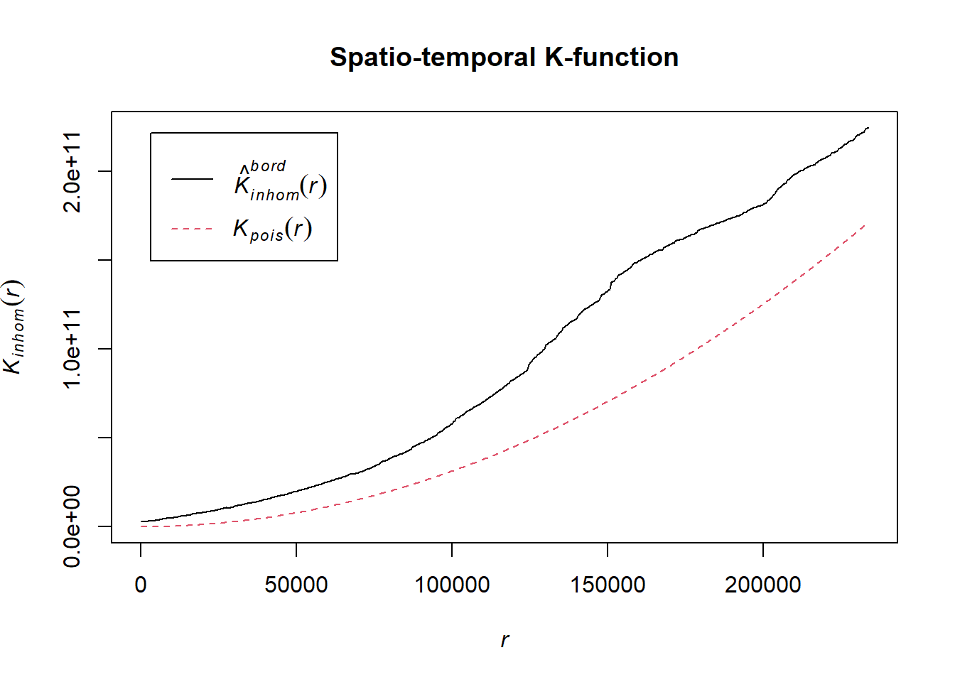
# Perform the CSR test with 99 simulations
K_ck.csr <- envelope(acled_spatio_ppp_owin, Kinhom, nsim=99, correction="border", parallel = parallel::detectCores())Generating 99 simulations of CSR ...
1, 2, [6:18 remaining] 3,
[6:12 remaining] 4, [6:04 remaining] 5, [6:00 remaining] 6,
[5:50 remaining] 7, [5:44 remaining] 8, [5:39 remaining] 9,
[5:33 remaining] 10, [5:29 remaining] 11, [5:27 remaining] 12,
[5:22 remaining] 13, [5:16 remaining] 14, [5:12 remaining] 15,
[5:11 remaining] 16, [5:08 remaining] 17, [5:04 remaining] 18,
[5:00 remaining] 19, [4:56 remaining] 20, [4:52 remaining] 21,
[4:50 remaining] 22, [4:48 remaining] 23, [4:45 remaining] 24,
[4:42 remaining] 25, [4:38 remaining] 26, [4:34 remaining] 27,
[4:30 remaining] 28, [4:26 remaining] 29, [4:22 remaining] 30,
[4:18 remaining] 31, [4:14 remaining] 32, [4:10 remaining] 33,
[4:06 remaining] 34, [4:02 remaining] 35, [3:58 remaining] 36,
[3:54 remaining] 37, [3:50 remaining] 38, [3:46 remaining] 39,
[3:43 remaining] 40, [3:39 remaining] 41, [3:35 remaining] 42,
[3:32 remaining] 43, [3:28 remaining] 44, [3:23 remaining] 45,
[3:19 remaining] 46, [3:14 remaining] 47, [3:10 remaining] 48,
[3:06 remaining] 49, [3:02 remaining] 50, [2:58 remaining] 51,
[2:54 remaining] 52, [2:50 remaining] 53, [2:46 remaining] 54,
[2:42 remaining] 55, [2:38 remaining] 56, [2:35 remaining] 57,
[2:31 remaining] 58, [2:27 remaining] 59, [2:23 remaining] 60,
[2:19 remaining] 61, [2:15 remaining] 62, [2:12 remaining] 63,
[2:08 remaining] 64, [2:04 remaining] 65, [2:01 remaining] 66,
[1:57 remaining] 67, [1:53 remaining] 68, [1:49 remaining] 69,
[1:46 remaining] 70, [1:42 remaining] 71, [1:39 remaining] 72,
[1:35 remaining] 73, [1:31 remaining] 74, [1:28 remaining] 75,
[1:24 remaining] 76, [1:20 remaining] 77, [1:17 remaining] 78,
[1:13 remaining] 79, [1:10 remaining] 80, [1:06 remaining] 81,
[1:03 remaining] 82, [59 sec remaining] 83, [56 sec remaining] 84,
[52 sec remaining] 85, [49 sec remaining] 86, [45 sec remaining] 87,
[42 sec remaining] 88, [38 sec remaining] 89, [35 sec remaining] 90,
[31 sec remaining] 91, [28 sec remaining] 92, [24 sec remaining] 93,
[21 sec remaining] 94, [17 sec remaining] 95, [14 sec remaining] 96,
[10 sec remaining] 97, [7 sec remaining] 98, [3 sec remaining]
99.
Done.# Plot the envelope with the observed K-function
plot(K_ck.csr, main="Spatio-temporal K-function Envelope", legend=TRUE)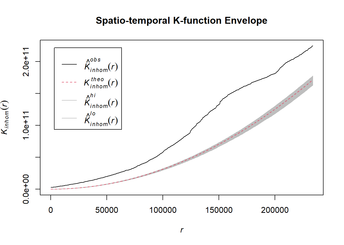
# Assuming `acled_spatio_ppp_owin` is your spatio-temporal point pattern object:
acled_spatio_ppp_owin <- acled_quarters_2022_ppp[regions_owin]
K_st <- Kinhom(acled_spatio_ppp_owin, correction="border")
# Plot the result for visual inspection
plot(K_st, main = "Spatio-temporal K-function", legend=TRUE)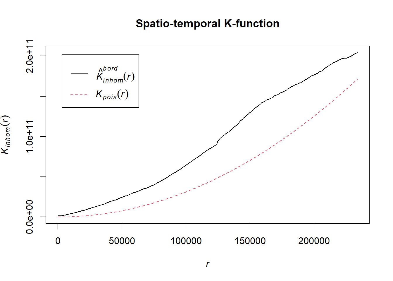
# Perform the CSR test with 99 simulations
K_ck.csr <- envelope(acled_spatio_ppp_owin, Kinhom, nsim=99, correction="border", parallel = parallel::detectCores())Generating 99 simulations of CSR ...
1, 2, [6:28 remaining] 3,
[6:24 remaining] 4, [6:20 remaining] 5, [6:18 remaining] 6,
[6:16 remaining] 7, [6:12 remaining] 8, [6:10 remaining] 9,
[6:07 remaining] 10, [6:02 remaining] 11, [5:59 remaining] 12,
[5:54 remaining] 13, [5:50 remaining] 14, [5:47 remaining] 15,
[5:42 remaining] 16, [5:38 remaining] 17, [5:35 remaining] 18,
[5:31 remaining] 19, [5:26 remaining] 20, [5:22 remaining] 21,
[5:17 remaining] 22, [5:14 remaining] 23, [5:09 remaining] 24,
[5:05 remaining] 25, [5:02 remaining] 26, [4:57 remaining] 27,
[4:53 remaining] 28, [4:49 remaining] 29, [4:45 remaining] 30,
[4:41 remaining] 31, [4:37 remaining] 32, [4:33 remaining] 33,
[4:29 remaining] 34, [4:25 remaining] 35, [4:21 remaining] 36,
[4:17 remaining] 37, [4:13 remaining] 38, [4:09 remaining] 39,
[4:05 remaining] 40, [4:01 remaining] 41, [3:57 remaining] 42,
[3:53 remaining] 43, [3:49 remaining] 44, [3:45 remaining] 45,
[3:41 remaining] 46, [3:37 remaining] 47, [3:32 remaining] 48,
[3:28 remaining] 49, [3:24 remaining] 50, [3:21 remaining] 51,
[3:16 remaining] 52, [3:12 remaining] 53, [3:08 remaining] 54,
[3:04 remaining] 55, [3:00 remaining] 56, [2:56 remaining] 57,
[2:52 remaining] 58, [2:48 remaining] 59, [2:44 remaining] 60,
[2:40 remaining] 61, [2:35 remaining] 62, [2:31 remaining] 63,
[2:27 remaining] 64, [2:23 remaining] 65, [2:19 remaining] 66,
[2:15 remaining] 67, [2:11 remaining] 68, [2:07 remaining] 69,
[2:03 remaining] 70, [1:58 remaining] 71, [1:54 remaining] 72,
[1:50 remaining] 73, [1:46 remaining] 74, [1:42 remaining] 75,
[1:38 remaining] 76, [1:34 remaining] 77, [1:30 remaining] 78,
[1:26 remaining] 79, [1:22 remaining] 80, [1:18 remaining] 81,
[1:14 remaining] 82, [1:10 remaining] 83, [1:05 remaining] 84,
[1:01 remaining] 85, [57 sec remaining] 86, [53 sec remaining] 87,
[49 sec remaining] 88, [45 sec remaining] 89, [41 sec remaining] 90,
[37 sec remaining] 91, [33 sec remaining] 92, [29 sec remaining] 93,
[25 sec remaining] 94, [20 sec remaining] 95, [16 sec remaining] 96,
[12 sec remaining] 97, [8 sec remaining] 98, [4 sec remaining]
99.
Done.# Plot the envelope with the observed K-function
plot(K_ck.csr, main="Spatio-temporal K-function Envelope", legend=TRUE)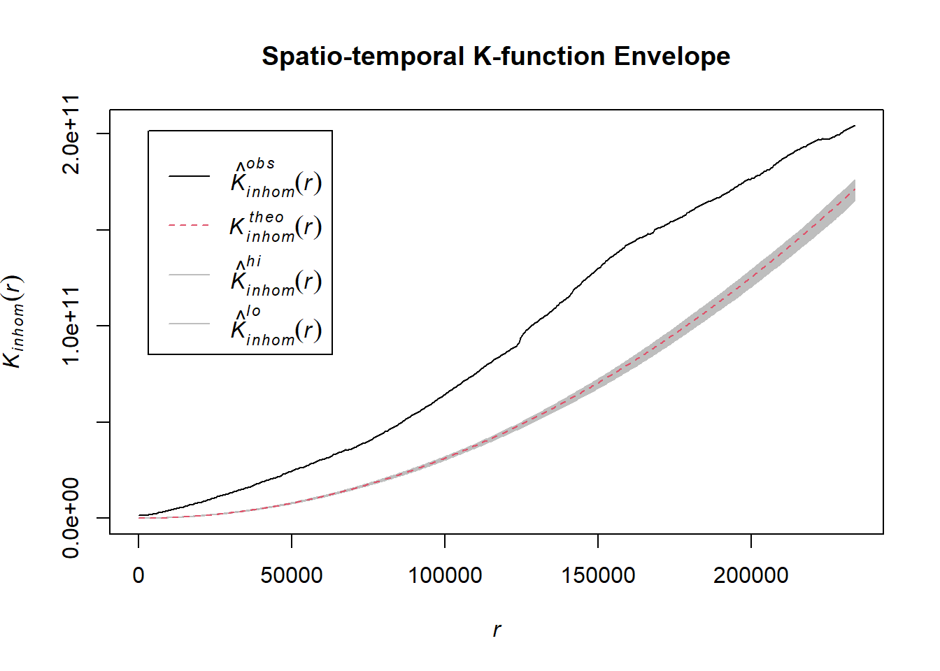
# Assuming `acled_spatio_ppp_owin` is your spatio-temporal point pattern object:
acled_spatio_ppp_owin <- acled_quarters_2023_ppp[regions_owin]
K_st <- Kinhom(acled_spatio_ppp_owin, correction="border")
# Plot the result for visual inspection
plot(K_st, main = "Spatio-temporal K-function", legend=TRUE)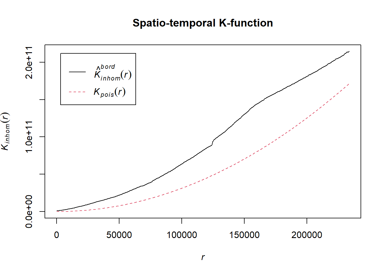
# Perform the CSR test with 99 simulations
K_ck.csr <- envelope(acled_spatio_ppp_owin, Kinhom, nsim=99, correction="border", parallel = parallel::detectCores())Generating 99 simulations of CSR ...
1, 2, [6:29 remaining] 3,
[6:28 remaining] 4, [6:21 remaining] 5, [6:22 remaining] 6,
[6:18 remaining] 7, [6:18 remaining] 8, [6:13 remaining] 9,
[6:08 remaining] 10, [6:06 remaining] 11, [6:02 remaining] 12,
[5:57 remaining] 13, [5:52 remaining] 14, [5:47 remaining] 15,
[5:42 remaining] 16, [5:40 remaining] 17, [5:35 remaining] 18,
[5:31 remaining] 19, [5:26 remaining] 20, [5:22 remaining] 21,
[5:17 remaining] 22, [5:13 remaining] 23, [5:09 remaining] 24,
[5:06 remaining] 25, [5:02 remaining] 26, [4:58 remaining] 27,
[4:54 remaining] 28, [4:50 remaining] 29, [4:45 remaining] 30,
[4:41 remaining] 31, [4:37 remaining] 32, [4:33 remaining] 33,
[4:30 remaining] 34, [4:26 remaining] 35, [4:21 remaining] 36,
[4:17 remaining] 37, [4:13 remaining] 38, [4:09 remaining] 39,
[4:05 remaining] 40, [4:01 remaining] 41, [3:57 remaining] 42,
[3:53 remaining] 43, [3:49 remaining] 44, [3:45 remaining] 45,
[3:41 remaining] 46, [3:37 remaining] 47, [3:33 remaining] 48,
[3:29 remaining] 49, [3:25 remaining] 50, [3:21 remaining] 51,
[3:17 remaining] 52, [3:13 remaining] 53, [3:09 remaining] 54,
[3:05 remaining] 55, [3:01 remaining] 56, [2:56 remaining] 57,
[2:52 remaining] 58, [2:48 remaining] 59, [2:44 remaining] 60,
[2:40 remaining] 61, [2:36 remaining] 62, [2:32 remaining] 63,
[2:28 remaining] 64, [2:23 remaining] 65, [2:19 remaining] 66,
[2:15 remaining] 67, [2:11 remaining] 68, [2:07 remaining] 69,
[2:03 remaining] 70, [1:59 remaining] 71, [1:55 remaining] 72,
[1:51 remaining] 73, [1:47 remaining] 74, [1:42 remaining] 75,
[1:38 remaining] 76, [1:34 remaining] 77, [1:30 remaining] 78,
[1:26 remaining] 79, [1:22 remaining] 80, [1:18 remaining] 81,
[1:14 remaining] 82, [1:10 remaining] 83, [1:06 remaining] 84,
[1:02 remaining] 85, [57 sec remaining] 86, [53 sec remaining] 87,
[49 sec remaining] 88, [45 sec remaining] 89, [41 sec remaining] 90,
[37 sec remaining] 91, [33 sec remaining] 92, [29 sec remaining] 93,
[25 sec remaining] 94, [21 sec remaining] 95, [16 sec remaining] 96,
[12 sec remaining] 97, [8 sec remaining] 98, [4 sec remaining]
99.
Done.# Plot the envelope with the observed K-function
plot(K_ck.csr, main="Spatio-temporal K-function Envelope", legend=TRUE)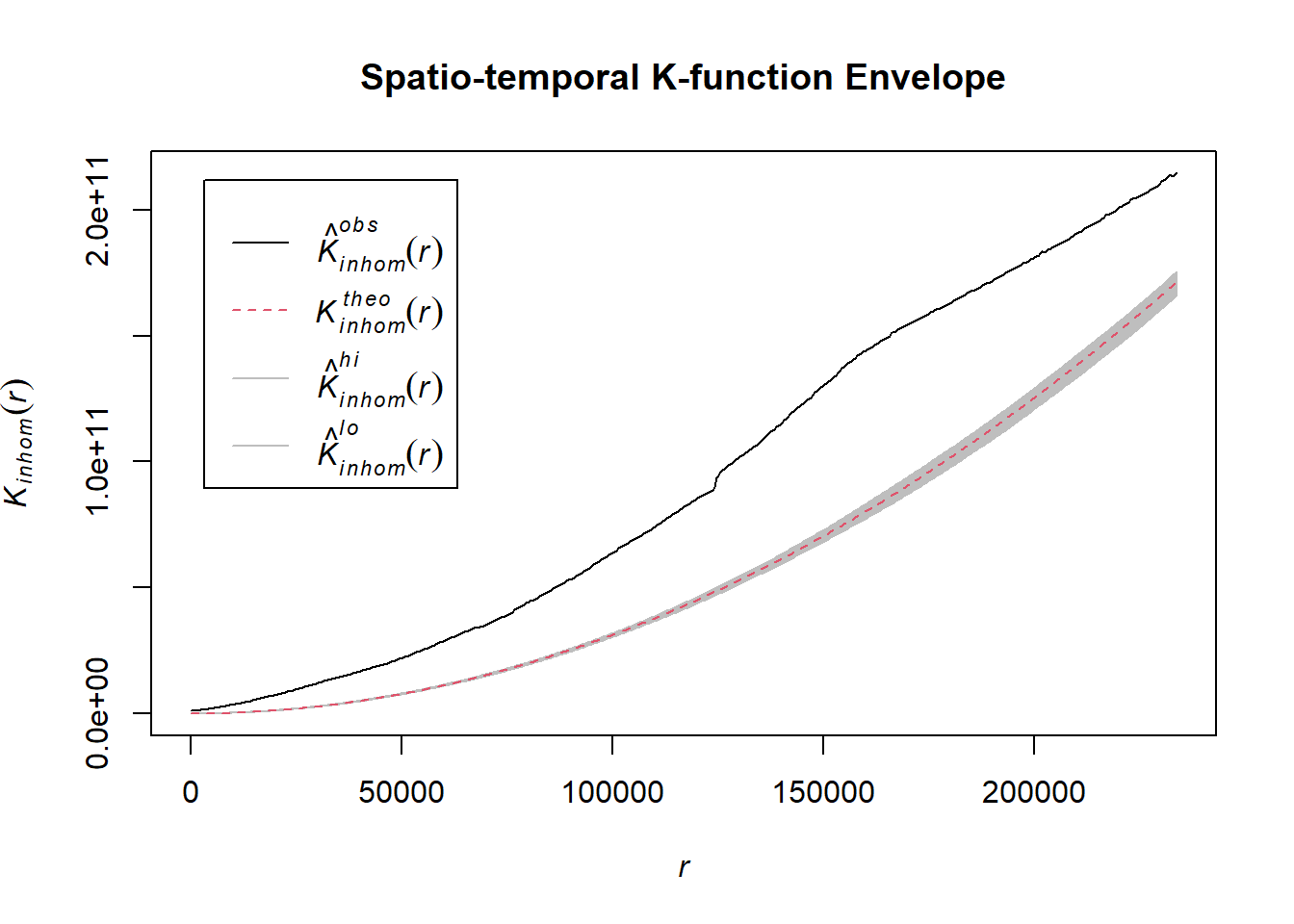
# Assuming `acled_spatio_ppp_owin` is your spatio-temporal point pattern object:
acled_spatio_ppp_owin <- acled_quarters_2024_ppp[regions_owin]
K_st <- Kinhom(acled_spatio_ppp_owin, correction="border")
# Plot the result for visual inspection
plot(K_st, main = "Spatio-temporal K-function", legend=TRUE)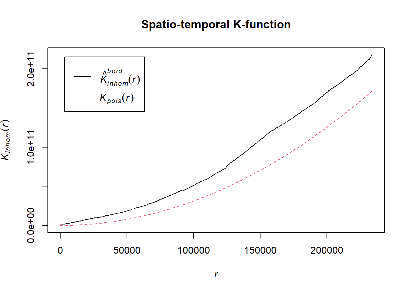
# Perform the CSR test with 99 simulations
K_ck.csr <- envelope(acled_spatio_ppp_owin, Kinhom, nsim=99, correction="border", parallel = parallel::detectCores())Generating 99 simulations of CSR ...
1, 2, [4:19 remaining] 3,
[4:12 remaining] 4, [4:10 remaining] 5, [4:09 remaining] 6,
[4:06 remaining] 7, [4:03 remaining] 8, [4:01 remaining] 9,
[3:58 remaining] 10, [3:58 remaining] 11, [3:54 remaining] 12,
[3:52 remaining] 13, [3:49 remaining] 14, [3:46 remaining] 15,
[3:43 remaining] 16, [3:41 remaining] 17, [3:38 remaining] 18,
[3:35 remaining] 19, [3:32 remaining] 20, [3:30 remaining] 21,
[3:28 remaining] 22, [3:25 remaining] 23, [3:23 remaining] 24,
[3:20 remaining] 25, [3:17 remaining] 26, [3:14 remaining] 27,
[3:12 remaining] 28, [3:09 remaining] 29, [3:06 remaining] 30,
[3:04 remaining] 31, [3:01 remaining] 32, [2:58 remaining] 33,
[2:58 remaining] 34, [2:56 remaining] 35, [2:53 remaining] 36,
[2:51 remaining] 37, [2:48 remaining] 38, [2:45 remaining] 39,
[2:42 remaining] 40, [2:40 remaining] 41, [2:37 remaining] 42,
[2:34 remaining] 43, [2:31 remaining] 44, [2:29 remaining] 45,
[2:26 remaining] 46, [2:23 remaining] 47, [2:20 remaining] 48,
[2:18 remaining] 49, [2:15 remaining] 50, [2:12 remaining] 51,
[2:09 remaining] 52, [2:07 remaining] 53, [2:04 remaining] 54,
[2:02 remaining] 55, [1:59 remaining] 56, [1:56 remaining] 57,
[1:53 remaining] 58, [1:50 remaining] 59, [1:48 remaining] 60,
[1:45 remaining] 61, [1:42 remaining] 62, [1:40 remaining] 63,
[1:37 remaining] 64, [1:34 remaining] 65, [1:32 remaining] 66,
[1:29 remaining] 67, [1:26 remaining] 68, [1:23 remaining] 69,
[1:21 remaining] 70, [1:18 remaining] 71, [1:15 remaining] 72,
[1:13 remaining] 73, [1:10 remaining] 74, [1:07 remaining] 75,
[1:05 remaining] 76, [1:02 remaining] 77, [59 sec remaining] 78,
[57 sec remaining] 79, [54 sec remaining] 80, [51 sec remaining] 81,
[48 sec remaining] 82, [46 sec remaining] 83, [43 sec remaining] 84,
[40 sec remaining] 85, [38 sec remaining] 86, [35 sec remaining] 87,
[32 sec remaining] 88, [30 sec remaining] 89, [27 sec remaining] 90,
[24 sec remaining] 91, [22 sec remaining] 92, [19 sec remaining] 93,
[16 sec remaining] 94, [13 sec remaining] 95, [11 sec remaining] 96,
[8 sec remaining] 97, [5 sec remaining] 98, [3 sec remaining]
99.
Done.# Plot the envelope with the observed K-function
plot(K_ck.csr, main="Spatio-temporal K-function Envelope", legend=TRUE)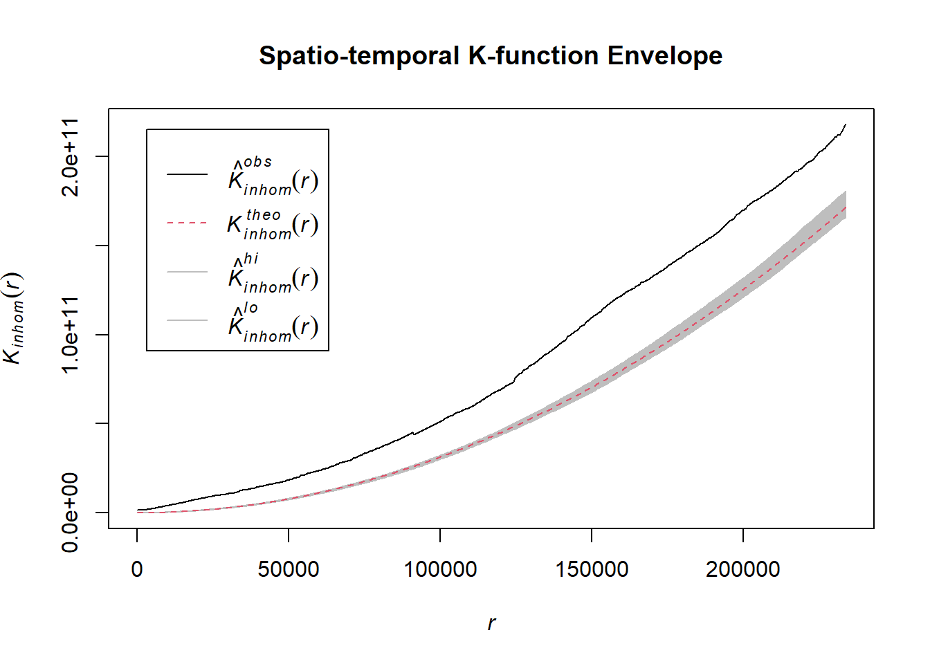
1.8.2 Strategic developments
# Assuming `acled_spatio_ppp_owin` is your spatio-temporal point pattern object:
acled_spatio_ppp_owin <- acled_quarters_2021_ppp[regions_owin]
K_st <- Kinhom(acled_spatio_ppp_owin, correction="border")
# Plot the result for visual inspection
plot(K_st, main = "Spatio-temporal K-function", legend=TRUE)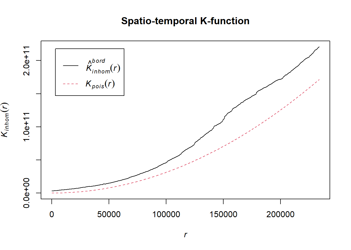
# Perform the CSR test with 99 simulations
K_ck.csr <- envelope(acled_spatio_ppp_owin, Kinhom, nsim=99, correction="border", parallel = parallel::detectCores())Generating 99 simulations of CSR ...
1, 2, [6:32 remaining] 3,
[6:15 remaining] 4, [6:07 remaining] 5, [6:08 remaining] 6,
[6:02 remaining] 7, [5:55 remaining] 8, [5:51 remaining] 9,
[5:47 remaining] 10, [5:42 remaining] 11, [5:38 remaining] 12,
[5:33 remaining] 13, [5:29 remaining] 14, [5:28 remaining] 15,
[5:23 remaining] 16, [5:20 remaining] 17, [5:16 remaining] 18,
[5:11 remaining] 19, [5:07 remaining] 20, [5:03 remaining] 21,
[4:58 remaining] 22, [4:54 remaining] 23, [4:51 remaining] 24,
[4:47 remaining] 25, [4:43 remaining] 26, [4:39 remaining] 27,
[4:35 remaining] 28, [4:32 remaining] 29, [4:28 remaining] 30,
[4:24 remaining] 31, [4:20 remaining] 32, [4:16 remaining] 33,
[4:12 remaining] 34, [4:08 remaining] 35, [4:04 remaining] 36,
[4:01 remaining] 37, [3:57 remaining] 38, [3:53 remaining] 39,
[3:50 remaining] 40, [3:46 remaining] 41, [3:42 remaining] 42,
[3:38 remaining] 43, [3:34 remaining] 44, [3:30 remaining] 45,
[3:26 remaining] 46, [3:23 remaining] 47, [3:19 remaining] 48,
[3:15 remaining] 49, [3:11 remaining] 50, [3:07 remaining] 51,
[3:03 remaining] 52, [2:59 remaining] 53, [2:56 remaining] 54,
[2:52 remaining] 55, [2:48 remaining] 56, [2:44 remaining] 57,
[2:41 remaining] 58, [2:37 remaining] 59, [2:33 remaining] 60,
[2:29 remaining] 61, [2:25 remaining] 62, [2:21 remaining] 63,
[2:17 remaining] 64, [2:14 remaining] 65, [2:10 remaining] 66,
[2:06 remaining] 67, [2:02 remaining] 68, [1:58 remaining] 69,
[1:54 remaining] 70, [1:51 remaining] 71, [1:47 remaining] 72,
[1:43 remaining] 73, [1:39 remaining] 74, [1:35 remaining] 75,
[1:32 remaining] 76, [1:28 remaining] 77, [1:24 remaining] 78,
[1:20 remaining] 79, [1:16 remaining] 80, [1:13 remaining] 81,
[1:09 remaining] 82, [1:05 remaining] 83, [1:01 remaining] 84,
[57 sec remaining] 85, [53 sec remaining] 86, [50 sec remaining] 87,
[46 sec remaining] 88, [42 sec remaining] 89, [38 sec remaining] 90,
[34 sec remaining] 91, [31 sec remaining] 92, [27 sec remaining] 93,
[23 sec remaining] 94, [19 sec remaining] 95, [15 sec remaining] 96,
[11 sec remaining] 97, [8 sec remaining] 98, [4 sec remaining]
99.
Done.# Plot the envelope with the observed K-function
plot(K_ck.csr, main="Spatio-temporal K-function Envelope", legend=TRUE)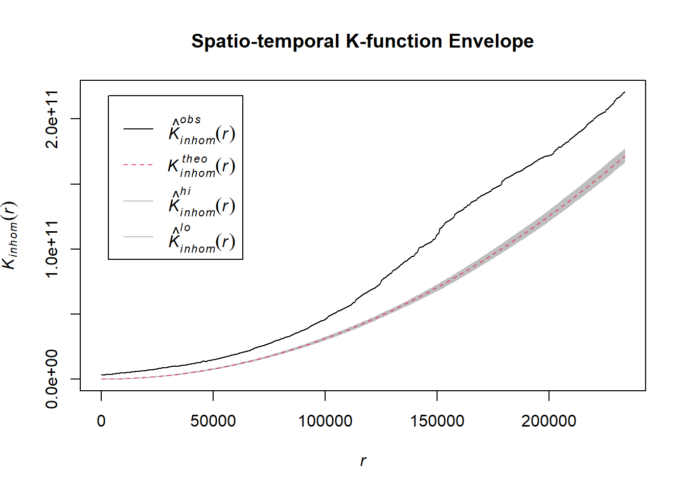
# Assuming `acled_spatio_ppp_owin` is your spatio-temporal point pattern object:
acled_spatio_ppp_owin <- acled_quarters_2022_ppp[regions_owin]
K_st <- Kinhom(acled_spatio_ppp_owin, correction="border")
# Plot the result for visual inspection
plot(K_st, main = "Spatio-temporal K-function", legend=TRUE)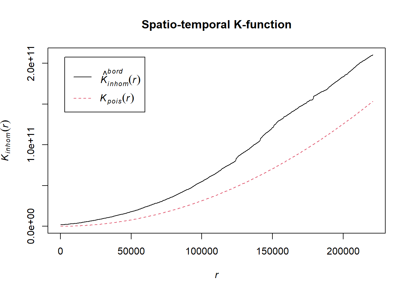
# Perform the CSR test with 99 simulations
K_ck.csr <- envelope(acled_spatio_ppp_owin, Kinhom, nsim=99, correction="border", parallel = parallel::detectCores())Generating 99 simulations of CSR ...
1, 2, [8:17 remaining] 3,
[8:00 remaining] 4, [7:52 remaining] 5, [7:40 remaining] 6,
[7:31 remaining] 7, [7:29 remaining] 8, [7:22 remaining] 9,
[7:15 remaining] 10, [7:10 remaining] 11, [7:05 remaining] 12,
[7:01 remaining] 13, [6:55 remaining] 14, [6:51 remaining] 15,
[6:48 remaining] 16, [6:42 remaining] 17, [6:37 remaining] 18,
[6:32 remaining] 19, [6:27 remaining] 20, [6:21 remaining] 21,
[6:16 remaining] 22, [6:11 remaining] 23, [6:07 remaining] 24,
[6:01 remaining] 25, [5:56 remaining] 26, [5:51 remaining] 27,
[5:46 remaining] 28, [5:42 remaining] 29, [5:37 remaining] 30,
[5:33 remaining] 31, [5:28 remaining] 32, [5:23 remaining] 33,
[5:18 remaining] 34, [5:13 remaining] 35, [5:09 remaining] 36,
[5:04 remaining] 37, [4:59 remaining] 38, [4:54 remaining] 39,
[4:49 remaining] 40, [4:44 remaining] 41, [4:39 remaining] 42,
[4:35 remaining] 43, [4:30 remaining] 44, [4:25 remaining] 45,
[4:20 remaining] 46, [4:15 remaining] 47, [4:10 remaining] 48,
[4:05 remaining] 49, [4:01 remaining] 50, [3:56 remaining] 51,
[3:51 remaining] 52, [3:46 remaining] 53, [3:41 remaining] 54,
[3:37 remaining] 55, [3:32 remaining] 56, [3:27 remaining] 57,
[3:22 remaining] 58, [3:17 remaining] 59, [3:12 remaining] 60,
[3:08 remaining] 61, [3:03 remaining] 62, [2:58 remaining] 63,
[2:53 remaining] 64, [2:48 remaining] 65, [2:43 remaining] 66,
[2:39 remaining] 67, [2:34 remaining] 68, [2:29 remaining] 69,
[2:24 remaining] 70, [2:19 remaining] 71, [2:15 remaining] 72,
[2:10 remaining] 73, [2:05 remaining] 74, [2:00 remaining] 75,
[1:55 remaining] 76, [1:51 remaining] 77, [1:46 remaining] 78,
[1:41 remaining] 79, [1:36 remaining] 80, [1:31 remaining] 81,
[1:27 remaining] 82, [1:22 remaining] 83, [1:17 remaining] 84,
[1:12 remaining] 85, [1:07 remaining] 86, [1:02 remaining] 87,
[58 sec remaining] 88, [53 sec remaining] 89, [48 sec remaining] 90,
[43 sec remaining] 91, [38 sec remaining] 92, [34 sec remaining] 93,
[29 sec remaining] 94, [24 sec remaining] 95, [19 sec remaining] 96,
[14 sec remaining] 97, [10 sec remaining] 98, [5 sec remaining]
99.
Done.# Plot the envelope with the observed K-function
plot(K_ck.csr, main="Spatio-temporal K-function Envelope", legend=TRUE)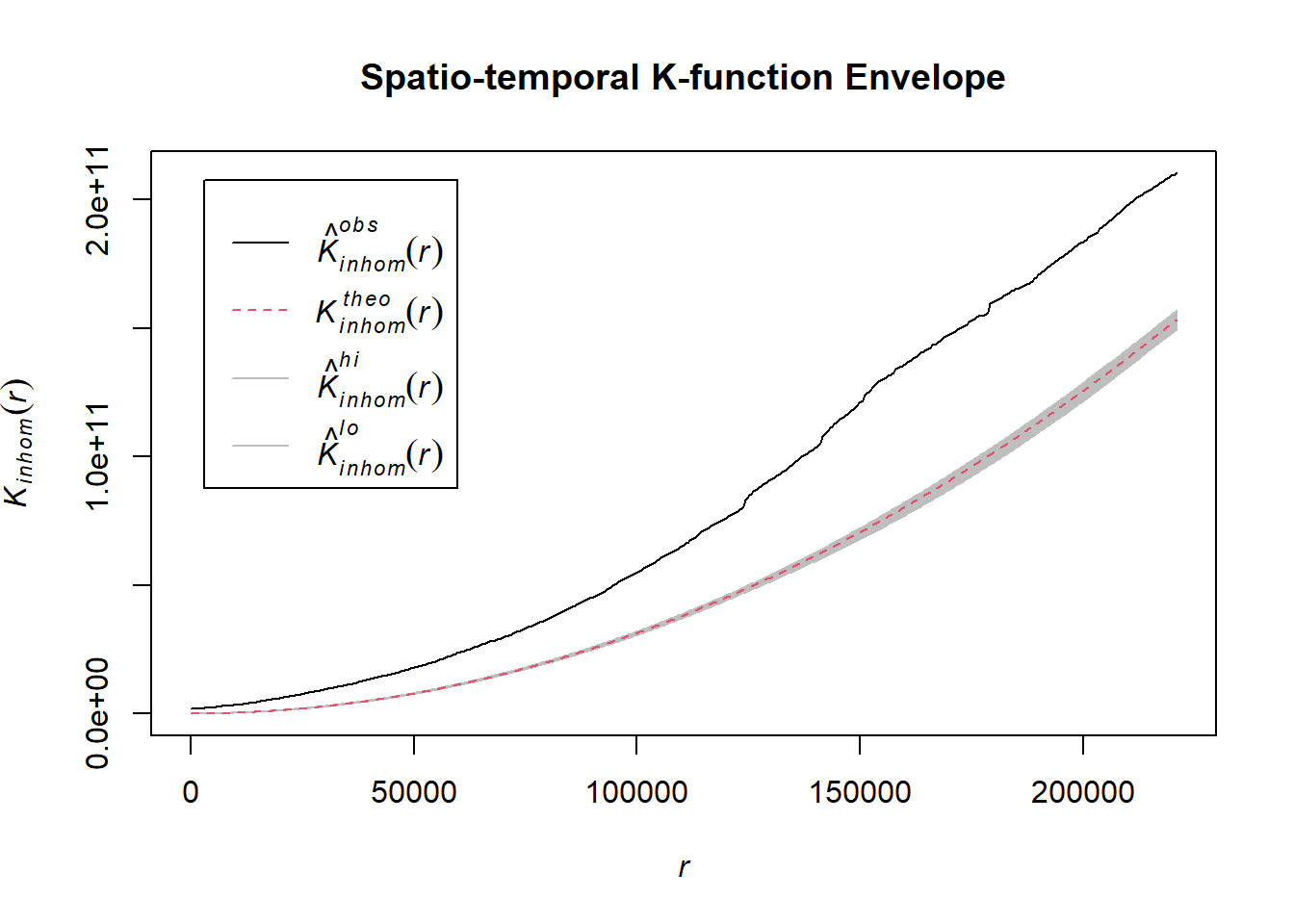
# Assuming `acled_spatio_ppp_owin` is your spatio-temporal point pattern object:
acled_spatio_ppp_owin <- acled_quarters_2023_ppp[regions_owin]
K_st <- Kinhom(acled_spatio_ppp_owin, correction="border")
# Plot the result for visual inspection
plot(K_st, main = "Spatio-temporal K-function", legend=TRUE)
# Perform the CSR test with 99 simulations
K_ck.csr <- envelope(acled_spatio_ppp_owin, Kinhom, nsim=99, correction="border", parallel = parallel::detectCores())Generating 99 simulations of CSR ...
1, 2, [5:53 remaining] 3,
[5:43 remaining] 4, [5:38 remaining] 5, [5:34 remaining] 6,
[5:39 remaining] 7, [5:32 remaining] 8, [5:27 remaining] 9,
[5:23 remaining] 10, [5:19 remaining] 11, [5:15 remaining] 12,
[5:11 remaining] 13, [5:08 remaining] 14, [5:04 remaining] 15,
[5:02 remaining] 16, [4:59 remaining] 17, [4:55 remaining] 18,
[4:51 remaining] 19, [4:47 remaining] 20, [4:44 remaining] 21,
[4:40 remaining] 22, [4:36 remaining] 23, [4:32 remaining] 24,
[4:29 remaining] 25, [4:26 remaining] 26, [4:22 remaining] 27,
[4:18 remaining] 28, [4:14 remaining] 29, [4:10 remaining] 30,
[4:07 remaining] 31, [4:03 remaining] 32, [3:59 remaining] 33,
[3:56 remaining] 34, [3:52 remaining] 35, [3:49 remaining] 36,
[3:45 remaining] 37, [3:41 remaining] 38, [3:38 remaining] 39,
[3:34 remaining] 40, [3:30 remaining] 41, [3:27 remaining] 42,
[3:23 remaining] 43, [3:20 remaining] 44, [3:16 remaining] 45,
[3:13 remaining] 46, [3:09 remaining] 47, [3:06 remaining] 48,
[3:02 remaining] 49, [2:58 remaining] 50, [2:55 remaining] 51,
[2:51 remaining] 52, [2:48 remaining] 53, [2:44 remaining] 54,
[2:41 remaining] 55, [2:37 remaining] 56, [2:33 remaining] 57,
[2:30 remaining] 58, [2:26 remaining] 59, [2:23 remaining] 60,
[2:19 remaining] 61, [2:16 remaining] 62, [2:12 remaining] 63,
[2:09 remaining] 64, [2:05 remaining] 65, [2:02 remaining] 66,
[1:58 remaining] 67, [1:54 remaining] 68, [1:51 remaining] 69,
[1:47 remaining] 70, [1:44 remaining] 71, [1:40 remaining] 72,
[1:37 remaining] 73, [1:33 remaining] 74, [1:29 remaining] 75,
[1:26 remaining] 76, [1:22 remaining] 77, [1:19 remaining] 78,
[1:15 remaining] 79, [1:12 remaining] 80, [1:08 remaining] 81,
[1:04 remaining] 82, [1:01 remaining] 83, [57 sec remaining] 84,
[54 sec remaining] 85, [50 sec remaining] 86, [47 sec remaining] 87,
[43 sec remaining] 88, [39 sec remaining] 89, [36 sec remaining] 90,
[32 sec remaining] 91, [29 sec remaining] 92, [25 sec remaining] 93,
[21 sec remaining] 94, [18 sec remaining] 95, [14 sec remaining] 96,
[11 sec remaining] 97, [7 sec remaining] 98, [4 sec remaining]
99.
Done.# Plot the envelope with the observed K-function
plot(K_ck.csr, main="Spatio-temporal K-function Envelope", legend=TRUE)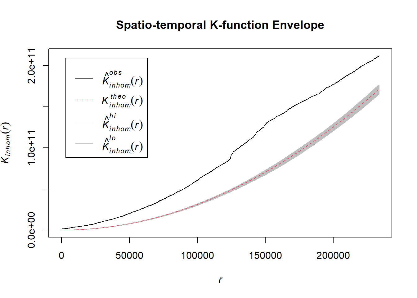
# Assuming `acled_spatio_ppp_owin` is your spatio-temporal point pattern object:
acled_spatio_ppp_owin <- acled_quarters_2024_ppp[regions_owin]
K_st <- Kinhom(acled_spatio_ppp_owin, correction="border")
# Plot the result for visual inspection
plot(K_st, main = "Spatio-temporal K-function", legend=TRUE)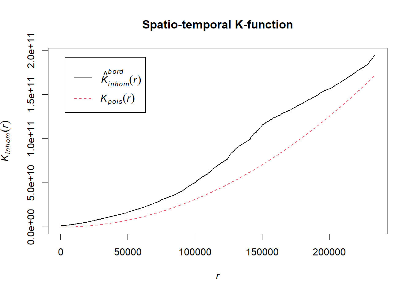
# Perform the CSR test with 99 simulations
K_ck.csr <- envelope(acled_spatio_ppp_owin, Kinhom, nsim=99, correction="border", parallel = parallel::detectCores())Generating 99 simulations of CSR ...
1, 2, [3:01 remaining] 3,
[3:02 remaining] 4, [3:00 remaining] 5, [2:55 remaining] 6,
[2:53 remaining] 7, [2:50 remaining] 8, [2:48 remaining] 9,
[2:47 remaining] 10, [2:44 remaining] 11, [2:44 remaining] 12,
[2:42 remaining] 13, [2:40 remaining] 14, [2:37 remaining] 15,
[2:35 remaining] 16, [2:33 remaining] 17, [2:31 remaining] 18,
[2:29 remaining] 19, [2:27 remaining] 20, [2:25 remaining] 21,
[2:23 remaining] 22, [2:21 remaining] 23, [2:20 remaining] 24,
[2:19 remaining] 25, [2:17 remaining] 26, [2:15 remaining] 27,
[2:13 remaining] 28, [2:11 remaining] 29, [2:09 remaining] 30,
[2:07 remaining] 31, [2:05 remaining] 32, [2:04 remaining] 33,
[2:02 remaining] 34, [2:00 remaining] 35, [1:58 remaining] 36,
[1:56 remaining] 37, [1:54 remaining] 38, [1:53 remaining] 39,
[1:51 remaining] 40, [1:50 remaining] 41, [1:48 remaining] 42,
[1:46 remaining] 43, [1:44 remaining] 44, [1:42 remaining] 45,
[1:40 remaining] 46, [1:38 remaining] 47, [1:36 remaining] 48,
[1:34 remaining] 49, [1:33 remaining] 50, [1:31 remaining] 51,
[1:29 remaining] 52, [1:27 remaining] 53, [1:25 remaining] 54,
[1:23 remaining] 55, [1:22 remaining] 56, [1:20 remaining] 57,
[1:18 remaining] 58, [1:16 remaining] 59, [1:14 remaining] 60,
[1:12 remaining] 61, [1:10 remaining] 62, [1:08 remaining] 63,
[1:07 remaining] 64, [1:05 remaining] 65, [1:03 remaining] 66,
[1:01 remaining] 67, [59 sec remaining] 68, [57 sec remaining] 69,
[55 sec remaining] 70, [54 sec remaining] 71, [52 sec remaining] 72,
[50 sec remaining] 73, [48 sec remaining] 74, [46 sec remaining] 75,
[44 sec remaining] 76, [43 sec remaining] 77, [41 sec remaining] 78,
[39 sec remaining] 79, [37 sec remaining] 80, [35 sec remaining] 81,
[33 sec remaining] 82, [31 sec remaining] 83, [30 sec remaining] 84,
[28 sec remaining] 85, [26 sec remaining] 86, [24 sec remaining] 87,
[22 sec remaining] 88, [20 sec remaining] 89, [18 sec remaining] 90,
[17 sec remaining] 91, [15 sec remaining] 92, [13 sec remaining] 93,
[11 sec remaining] 94, [9 sec remaining] 95, [7 sec remaining] 96,
[6 sec remaining] 97, [4 sec remaining] 98, [2 sec remaining]
99.
Done.# Plot the envelope with the observed K-function
plot(K_ck.csr, main="Spatio-temporal K-function Envelope", legend=TRUE)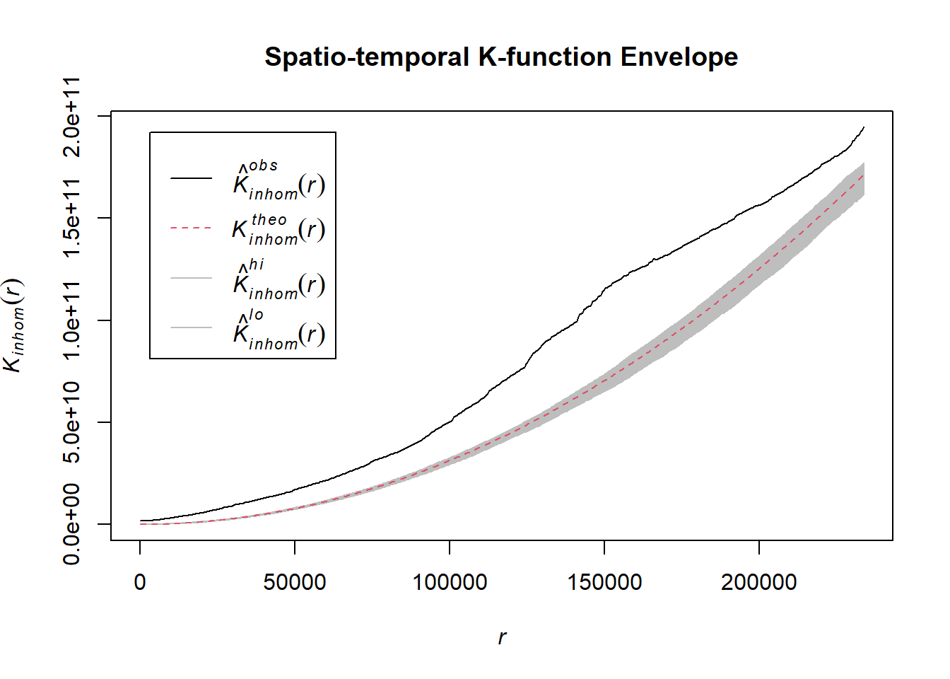
1.8.3 Battles
# Assuming `acled_spatio_ppp_owin` is your spatio-temporal point pattern object:
acled_spatio_ppp_owin <- acled_quarters_2021_ppp[regions_owin]
K_st <- Kinhom(acled_spatio_ppp_owin, correction="border")
# Plot the result for visual inspection
plot(K_st, main = "Spatio-temporal K-function", legend=TRUE)
# Perform the CSR test with 99 simulations
K_ck.csr <- envelope(acled_spatio_ppp_owin, Kinhom, nsim=99, correction="border", parallel = parallel::detectCores())Generating 99 simulations of CSR ...
1, 2, [4:38 remaining] 3,
[4:30 remaining] 4, [4:27 remaining] 5, [4:28 remaining] 6,
[4:22 remaining] 7, [4:17 remaining] 8, [4:12 remaining] 9,
[4:08 remaining] 10, [4:05 remaining] 11, [4:03 remaining] 12,
[3:59 remaining] 13, [3:56 remaining] 14, [3:57 remaining] 15,
[3:57 remaining] 16, [3:57 remaining] 17, [3:57 remaining] 18,
[3:53 remaining] 19, [3:50 remaining] 20, [3:46 remaining] 21,
[3:44 remaining] 22, [3:40 remaining] 23, [3:37 remaining] 24,
[3:34 remaining] 25, [3:31 remaining] 26, [3:28 remaining] 27,
[3:24 remaining] 28, [3:22 remaining] 29, [3:19 remaining] 30,
[3:16 remaining] 31, [3:13 remaining] 32, [3:10 remaining] 33,
[3:07 remaining] 34, [3:04 remaining] 35, [3:01 remaining] 36,
[2:58 remaining] 37, [2:55 remaining] 38, [2:53 remaining] 39,
[2:50 remaining] 40, [2:47 remaining] 41, [2:44 remaining] 42,
[2:41 remaining] 43, [2:38 remaining] 44, [2:35 remaining] 45,
[2:32 remaining] 46, [2:29 remaining] 47, [2:26 remaining] 48,
[2:24 remaining] 49, [2:21 remaining] 50, [2:18 remaining] 51,
[2:15 remaining] 52, [2:12 remaining] 53, [2:09 remaining] 54,
[2:06 remaining] 55, [2:04 remaining] 56, [2:01 remaining] 57,
[1:58 remaining] 58, [1:55 remaining] 59, [1:52 remaining] 60,
[1:49 remaining] 61, [1:47 remaining] 62, [1:44 remaining] 63,
[1:41 remaining] 64, [1:38 remaining] 65, [1:35 remaining] 66,
[1:33 remaining] 67, [1:30 remaining] 68, [1:27 remaining] 69,
[1:24 remaining] 70, [1:21 remaining] 71, [1:19 remaining] 72,
[1:16 remaining] 73, [1:13 remaining] 74, [1:10 remaining] 75,
[1:07 remaining] 76, [1:04 remaining] 77, [1:02 remaining] 78,
[59 sec remaining] 79, [56 sec remaining] 80, [53 sec remaining] 81,
[50 sec remaining] 82, [48 sec remaining] 83, [45 sec remaining] 84,
[42 sec remaining] 85, [39 sec remaining] 86, [36 sec remaining] 87,
[34 sec remaining] 88, [31 sec remaining] 89, [28 sec remaining] 90,
[25 sec remaining] 91, [22 sec remaining] 92, [20 sec remaining] 93,
[17 sec remaining] 94, [14 sec remaining] 95, [11 sec remaining] 96,
[8 sec remaining] 97, [6 sec remaining] 98, [3 sec remaining]
99.
Done.# Plot the envelope with the observed K-function
plot(K_ck.csr, main="Spatio-temporal K-function Envelope", legend=TRUE)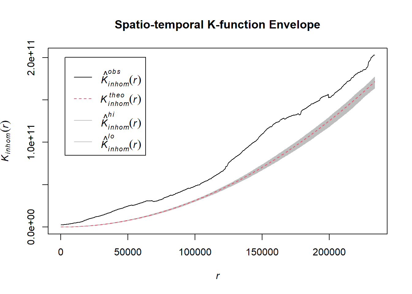
# Assuming `acled_spatio_ppp_owin` is your spatio-temporal point pattern object:
acled_spatio_ppp_owin <- acled_quarters_2022_ppp[regions_owin]
K_st <- Kinhom(acled_spatio_ppp_owin, correction="border")
# Plot the result for visual inspection
plot(K_st, main = "Spatio-temporal K-function", legend=TRUE)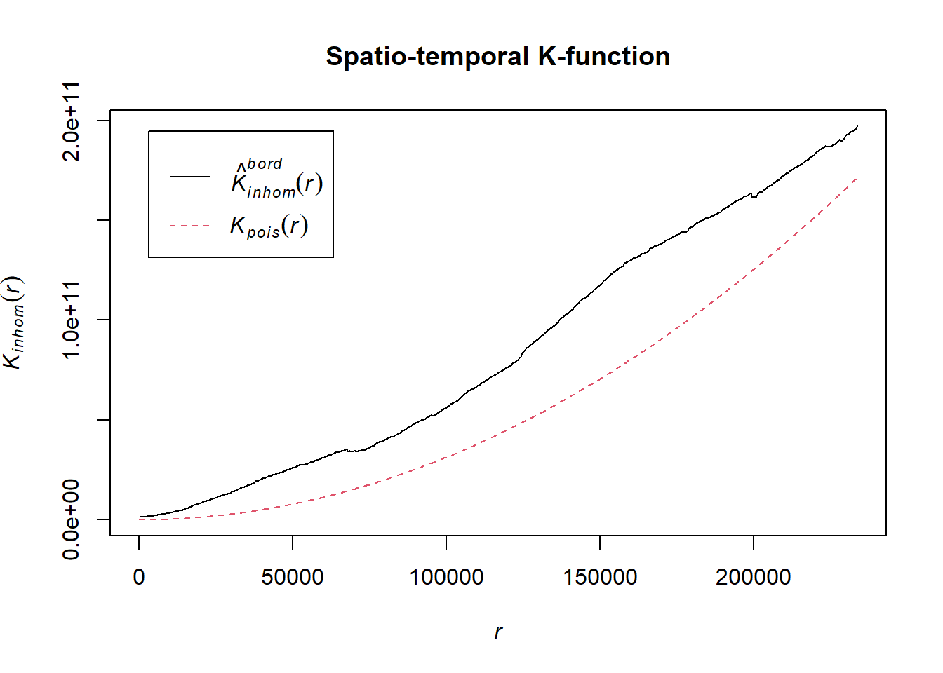
# Perform the CSR test with 99 simulations
K_ck.csr <- envelope(acled_spatio_ppp_owin, Kinhom, nsim=99, correction="border", parallel = parallel::detectCores())Generating 99 simulations of CSR ...
1, 2, [6:54 remaining] 3,
[7:37 remaining] 4, [7:24 remaining] 5, [7:09 remaining] 6,
[7:00 remaining] 7, [6:54 remaining] 8, [6:47 remaining] 9,
[6:44 remaining] 10, [6:45 remaining] 11, [6:43 remaining] 12,
[6:37 remaining] 13, [6:30 remaining] 14, [6:25 remaining] 15,
[6:18 remaining] 16, [6:12 remaining] 17, [6:06 remaining] 18,
[6:02 remaining] 19, [5:56 remaining] 20, [5:51 remaining] 21,
[5:46 remaining] 22, [5:41 remaining] 23, [5:35 remaining] 24,
[5:31 remaining] 25, [5:27 remaining] 26, [5:23 remaining] 27,
[5:18 remaining] 28, [5:13 remaining] 29, [5:08 remaining] 30,
[5:04 remaining] 31, [4:59 remaining] 32, [4:54 remaining] 33,
[4:49 remaining] 34, [4:45 remaining] 35, [4:40 remaining] 36,
[4:36 remaining] 37, [4:31 remaining] 38, [4:26 remaining] 39,
[4:22 remaining] 40, [4:17 remaining] 41, [4:14 remaining] 42,
[4:09 remaining] 43, [4:05 remaining] 44, [4:00 remaining] 45,
[3:56 remaining] 46, [3:51 remaining] 47, [3:47 remaining] 48,
[3:43 remaining] 49, [3:39 remaining] 50, [3:35 remaining] 51,
[3:31 remaining] 52, [3:26 remaining] 53, [3:22 remaining] 54,
[3:18 remaining] 55, [3:14 remaining] 56, [3:10 remaining] 57,
[3:06 remaining] 58, [3:01 remaining] 59, [2:57 remaining] 60,
[2:53 remaining] 61, [2:48 remaining] 62, [2:43 remaining] 63,
[2:39 remaining] 64, [2:34 remaining] 65, [2:30 remaining] 66,
[2:26 remaining] 67, [2:21 remaining] 68, [2:17 remaining] 69,
[2:12 remaining] 70, [2:08 remaining] 71, [2:03 remaining] 72,
[1:59 remaining] 73, [1:54 remaining] 74, [1:50 remaining] 75,
[1:46 remaining] 76, [1:41 remaining] 77, [1:37 remaining] 78,
[1:33 remaining] 79, [1:28 remaining] 80, [1:24 remaining] 81,
[1:20 remaining] 82, [1:15 remaining] 83, [1:11 remaining] 84,
[1:06 remaining] 85, [1:02 remaining] 86, [57 sec remaining] 87,
[53 sec remaining] 88, [49 sec remaining] 89, [44 sec remaining] 90,
[40 sec remaining] 91, [35 sec remaining] 92, [31 sec remaining] 93,
[26 sec remaining] 94, [22 sec remaining] 95, [18 sec remaining] 96,
[13 sec remaining] 97, [9 sec remaining] 98, [4 sec remaining]
99.
Done.# Plot the envelope with the observed K-function
plot(K_ck.csr, main="Spatio-temporal K-function Envelope", legend=TRUE)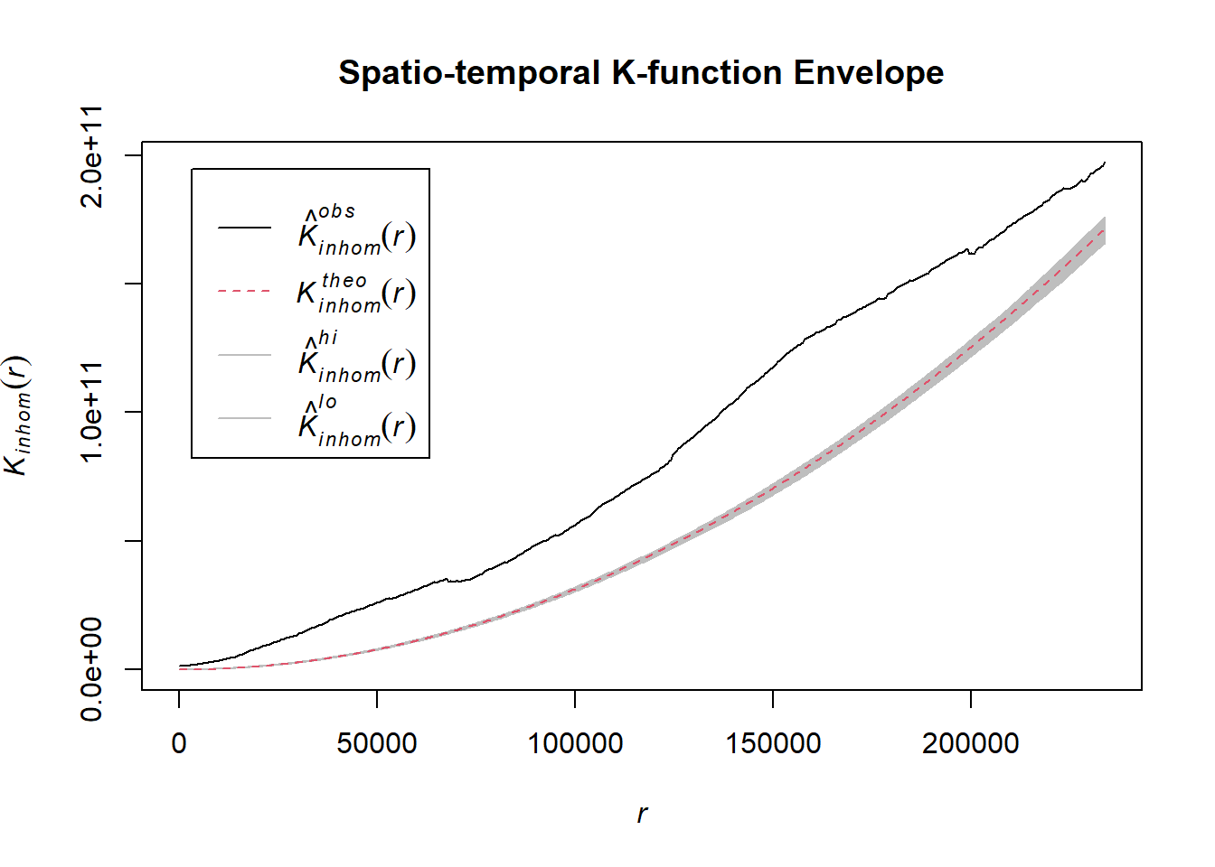
# Assuming `acled_spatio_ppp_owin` is your spatio-temporal point pattern object:
acled_spatio_ppp_owin <- acled_quarters_2023_ppp[regions_owin]
K_st <- Kinhom(acled_spatio_ppp_owin, correction="border")
# Plot the result for visual inspection
plot(K_st, main = "Spatio-temporal K-function", legend=TRUE)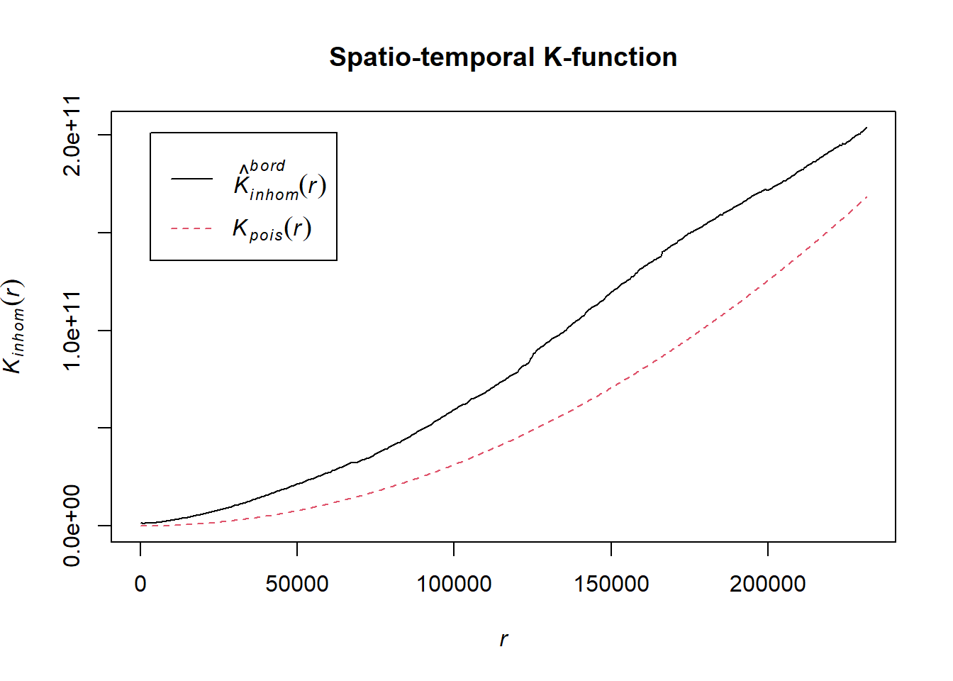
# Perform the CSR test with 99 simulations
K_ck.csr <- envelope(acled_spatio_ppp_owin, Kinhom, nsim=99, correction="border", parallel = parallel::detectCores())Generating 99 simulations of CSR ...
1, 2, [7:05 remaining] 3,
[7:23 remaining] 4, [7:22 remaining] 5, [7:11 remaining] 6,
[7:18 remaining] 7, [7:26 remaining] 8, [7:19 remaining] 9,
[7:11 remaining] 10, [7:02 remaining] 11, [6:54 remaining] 12,
[6:51 remaining] 13, [6:45 remaining] 14, [6:38 remaining] 15,
[6:34 remaining] 16, [6:27 remaining] 17, [6:20 remaining] 18,
[6:14 remaining] 19, [6:08 remaining] 20, [6:03 remaining] 21,
[5:57 remaining] 22, [5:52 remaining] 23, [5:48 remaining] 24,
[5:43 remaining] 25, [5:38 remaining] 26, [5:33 remaining] 27,
[5:27 remaining] 28, [5:22 remaining] 29, [5:18 remaining] 30,
[5:13 remaining] 31, [5:08 remaining] 32, [5:03 remaining] 33,
[4:59 remaining] 34, [4:54 remaining] 35, [4:49 remaining] 36,
[4:44 remaining] 37, [4:39 remaining] 38, [4:34 remaining] 39,
[4:30 remaining] 40, [4:26 remaining] 41, [4:21 remaining] 42,
[4:16 remaining] 43, [4:12 remaining] 44, [4:07 remaining] 45,
[4:02 remaining] 46, [3:58 remaining] 47, [3:53 remaining] 48,
[3:49 remaining] 49, [3:44 remaining] 50, [3:40 remaining] 51,
[3:35 remaining] 52, [3:30 remaining] 53, [3:26 remaining] 54,
[3:21 remaining] 55, [3:17 remaining] 56, [3:12 remaining] 57,
[3:08 remaining] 58, [3:03 remaining] 59, [2:59 remaining] 60,
[2:54 remaining] 61, [2:50 remaining] 62, [2:45 remaining] 63,
[2:41 remaining] 64, [2:36 remaining] 65, [2:32 remaining] 66,
[2:27 remaining] 67, [2:23 remaining] 68, [2:18 remaining] 69,
[2:14 remaining] 70, [2:09 remaining] 71, [2:05 remaining] 72,
[2:00 remaining] 73, [1:56 remaining] 74, [1:51 remaining] 75,
[1:47 remaining] 76, [1:42 remaining] 77, [1:38 remaining] 78,
[1:33 remaining] 79, [1:29 remaining] 80, [1:24 remaining] 81,
[1:20 remaining] 82, [1:16 remaining] 83, [1:11 remaining] 84,
[1:07 remaining] 85, [1:02 remaining] 86, [58 sec remaining] 87,
[53 sec remaining] 88, [49 sec remaining] 89, [45 sec remaining] 90,
[40 sec remaining] 91, [36 sec remaining] 92, [31 sec remaining] 93,
[27 sec remaining] 94, [22 sec remaining] 95, [18 sec remaining] 96,
[13 sec remaining] 97, [9 sec remaining] 98, [4 sec remaining]
99.
Done.# Plot the envelope with the observed K-function
plot(K_ck.csr, main="Spatio-temporal K-function Envelope", legend=TRUE)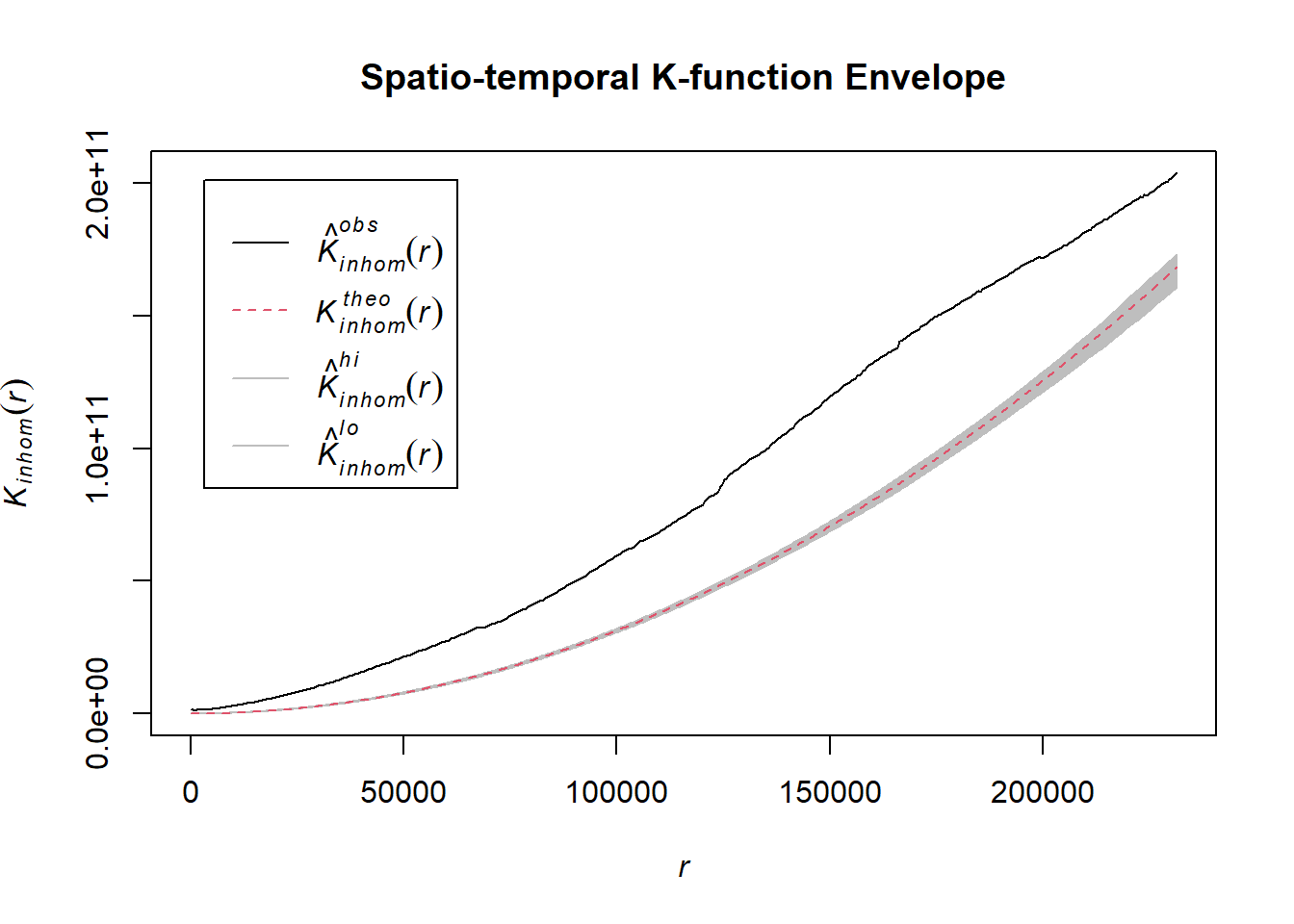
# Assuming `acled_spatio_ppp_owin` is your spatio-temporal point pattern object:
acled_spatio_ppp_owin <- acled_quarters_2024_ppp[regions_owin]
K_st <- Kinhom(acled_spatio_ppp_owin, correction="border")
# Plot the result for visual inspection
plot(K_st, main = "Spatio-temporal K-function", legend=TRUE)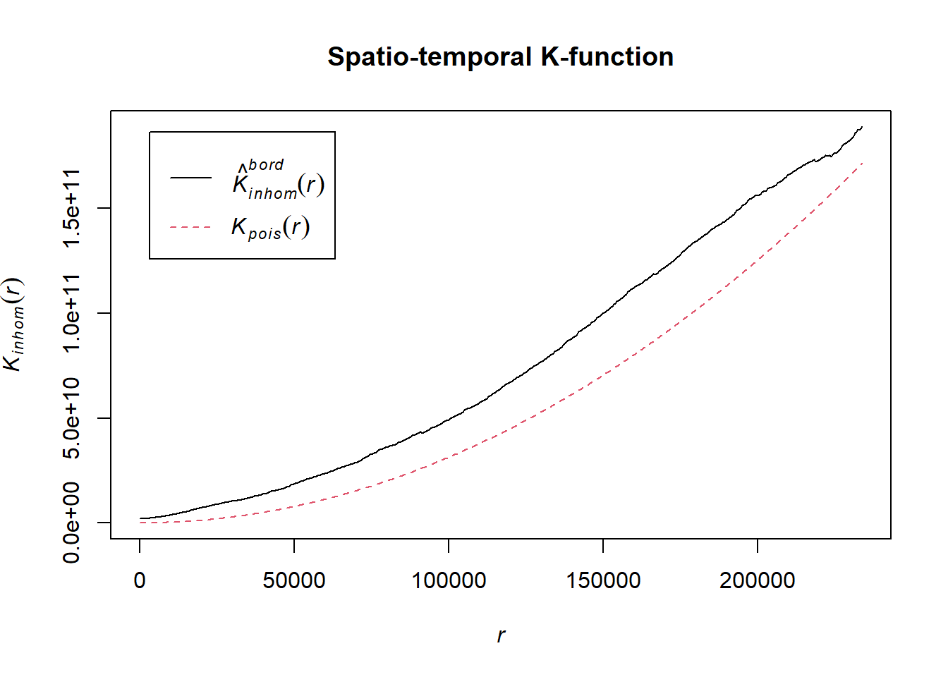
# Perform the CSR test with 99 simulations
K_ck.csr <- envelope(acled_spatio_ppp_owin, Kinhom, nsim=50, correction="border", parallel = parallel::detectCores())Generating 50 simulations of CSR ...
1, 2, 3, 4, 5, 6, 7, 8, 9, 10, 11, 12, 13, 14, 15, 16, 17, 18, 19, 20,
21, 22, 23, 24, 25, 26, 27, 28, 29, 30, 31, 32, 33, 34, 35, 36, 37, 38, 39, 40,
41, 42, 43, 44, 45, 46, 47, 48, 49,
50.
Done.# Plot the envelope with the observed K-function
plot(K_ck.csr, main="Spatio-temporal K-function Envelope", legend=TRUE)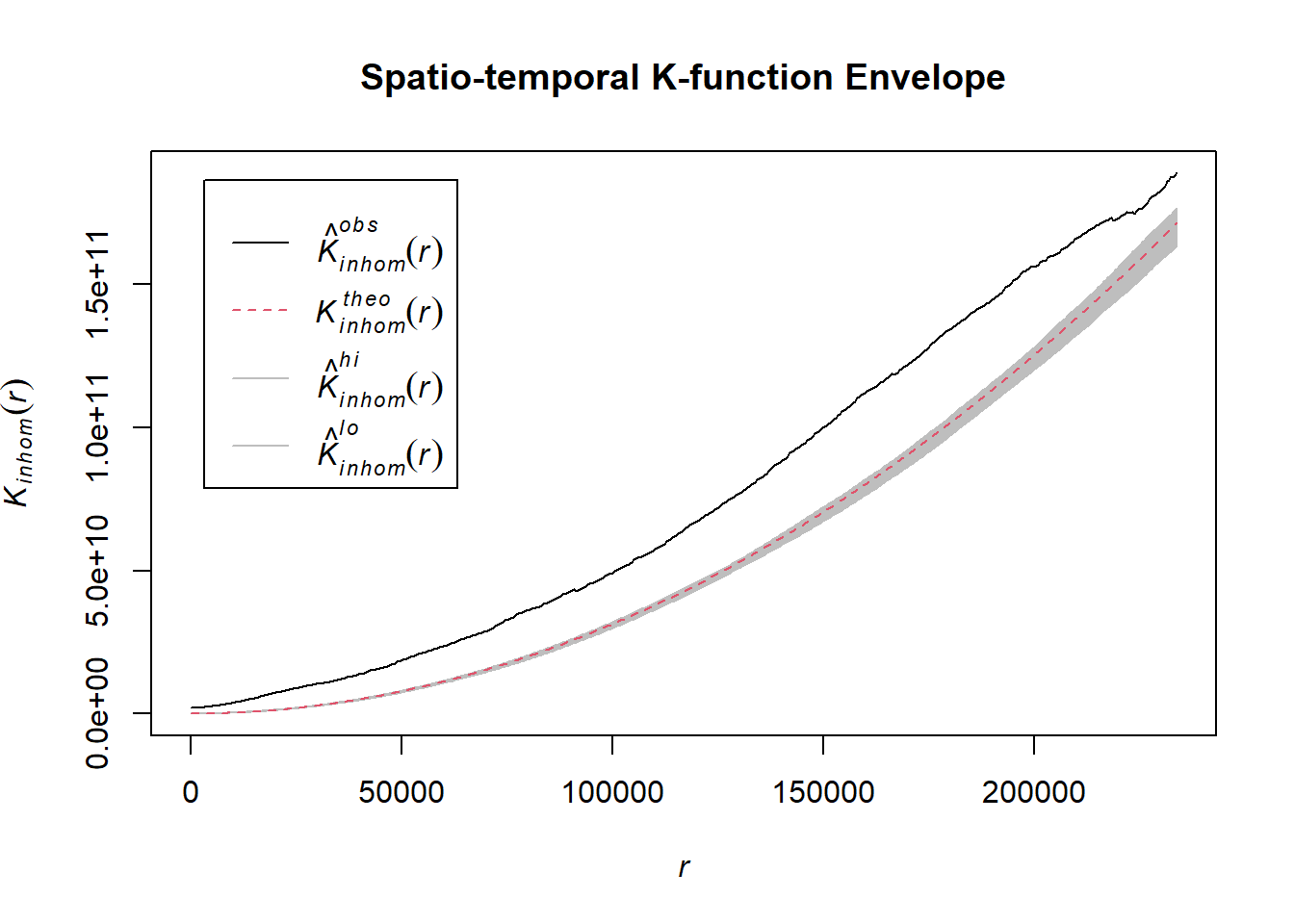
1.8.3 Violence against civilians
# Assuming `acled_spatio_ppp_owin` is your spatio-temporal point pattern object:
acled_spatio_ppp_owin <- acled_quarters_2021_ppp[regions_owin]
K_st <- Kinhom(acled_spatio_ppp_owin, correction="border")
# Plot the result for visual inspection
plot(K_st, main = "Spatio-temporal K-function", legend=TRUE)
# Perform the CSR test with 99 simulations
K_ck.csr <- envelope(acled_spatio_ppp_owin, Kinhom, nsim=99, correction="border", parallel = parallel::detectCores())Generating 99 simulations of CSR ...
1, 2, [3:52 remaining] 3,
[3:49 remaining] 4, [3:48 remaining] 5, [3:47 remaining] 6,
[3:43 remaining] 7, [3:42 remaining] 8, [3:38 remaining] 9,
[3:41 remaining] 10, [3:38 remaining] 11, [3:35 remaining] 12,
[3:32 remaining] 13, [3:29 remaining] 14, [3:26 remaining] 15,
[3:23 remaining] 16, [3:21 remaining] 17, [3:18 remaining] 18,
[3:16 remaining] 19, [3:13 remaining] 20, [3:11 remaining] 21,
[3:09 remaining] 22, [3:07 remaining] 23, [3:04 remaining] 24,
[3:02 remaining] 25, [2:59 remaining] 26, [2:57 remaining] 27,
[2:55 remaining] 28, [2:52 remaining] 29, [2:50 remaining] 30,
[2:47 remaining] 31, [2:45 remaining] 32, [2:42 remaining] 33,
[2:40 remaining] 34, [2:38 remaining] 35, [2:35 remaining] 36,
[2:33 remaining] 37, [2:30 remaining] 38, [2:28 remaining] 39,
[2:25 remaining] 40, [2:23 remaining] 41, [2:20 remaining] 42,
[2:18 remaining] 43, [2:15 remaining] 44, [2:13 remaining] 45,
[2:11 remaining] 46, [2:08 remaining] 47, [2:06 remaining] 48,
[2:03 remaining] 49, [2:01 remaining] 50, [1:59 remaining] 51,
[1:56 remaining] 52, [1:54 remaining] 53, [1:51 remaining] 54,
[1:49 remaining] 55, [1:46 remaining] 56, [1:44 remaining] 57,
[1:42 remaining] 58, [1:40 remaining] 59, [1:37 remaining] 60,
[1:35 remaining] 61, [1:32 remaining] 62, [1:30 remaining] 63,
[1:27 remaining] 64, [1:25 remaining] 65, [1:24 remaining] 66,
[1:21 remaining] 67, [1:19 remaining] 68, [1:17 remaining] 69,
[1:15 remaining] 70, [1:12 remaining] 71, [1:10 remaining] 72,
[1:07 remaining] 73, [1:05 remaining] 74, [1:02 remaining] 75,
[1:00 remaining] 76, [57 sec remaining] 77, [55 sec remaining] 78,
[53 sec remaining] 79, [50 sec remaining] 80, [48 sec remaining] 81,
[45 sec remaining] 82, [43 sec remaining] 83, [40 sec remaining] 84,
[38 sec remaining] 85, [35 sec remaining] 86, [33 sec remaining] 87,
[30 sec remaining] 88, [28 sec remaining] 89, [25 sec remaining] 90,
[22 sec remaining] 91, [20 sec remaining] 92, [17 sec remaining] 93,
[15 sec remaining] 94, [12 sec remaining] 95, [10 sec remaining] 96,
[8 sec remaining] 97, [5 sec remaining] 98, [3 sec remaining]
99.
Done.# Plot the envelope with the observed K-function
plot(K_ck.csr, main="Spatio-temporal K-function Envelope", legend=TRUE)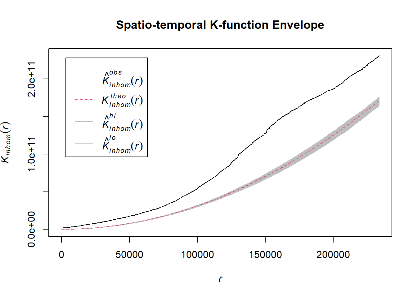
# Assuming `acled_spatio_ppp_owin` is your spatio-temporal point pattern object:
acled_spatio_ppp_owin <- acled_quarters_2022_ppp[regions_owin]
K_st <- Kinhom(acled_spatio_ppp_owin, correction="border")
# Plot the result for visual inspection
plot(K_st, main = "Spatio-temporal K-function", legend=TRUE)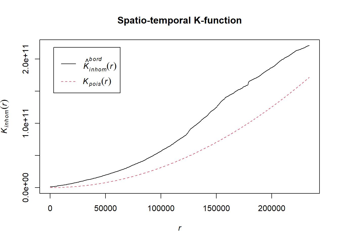
# Perform the CSR test with 99 simulations
K_ck.csr <- envelope(acled_spatio_ppp_owin, Kinhom, nsim=99, correction="border", parallel = parallel::detectCores())Generating 99 simulations of CSR ...
1, 2, [4:25 remaining] 3,
[4:21 remaining] 4, [4:28 remaining] 5, [4:19 remaining] 6,
[4:15 remaining] 7, [4:09 remaining] 8, [4:05 remaining] 9,
[4:01 remaining] 10, [4:06 remaining] 11, [4:03 remaining] 12,
[4:01 remaining] 13, [3:58 remaining] 14, [3:55 remaining] 15,
[3:54 remaining] 16, [3:50 remaining] 17, [3:46 remaining] 18,
[3:46 remaining] 19, [3:43 remaining] 20, [3:39 remaining] 21,
[3:37 remaining] 22, [3:34 remaining] 23, [3:31 remaining] 24,
[3:29 remaining] 25, [3:26 remaining] 26, [3:24 remaining] 27,
[3:23 remaining] 28, [3:22 remaining] 29, [3:20 remaining] 30,
[3:17 remaining] 31, [3:14 remaining] 32, [3:11 remaining] 33,
[3:08 remaining] 34, [3:05 remaining] 35, [3:01 remaining] 36,
[2:58 remaining] 37, [2:55 remaining] 38, [2:52 remaining] 39,
[2:49 remaining] 40, [2:46 remaining] 41, [2:43 remaining] 42,
[2:40 remaining] 43, [2:38 remaining] 44, [2:35 remaining] 45,
[2:32 remaining] 46, [2:28 remaining] 47, [2:26 remaining] 48,
[2:22 remaining] 49, [2:19 remaining] 50, [2:17 remaining] 51,
[2:14 remaining] 52, [2:11 remaining] 53, [2:08 remaining] 54,
[2:05 remaining] 55, [2:02 remaining] 56, [1:59 remaining] 57,
[1:56 remaining] 58, [1:53 remaining] 59, [1:50 remaining] 60,
[1:47 remaining] 61, [1:45 remaining] 62, [1:42 remaining] 63,
[1:39 remaining] 64, [1:36 remaining] 65, [1:33 remaining] 66,
[1:30 remaining] 67, [1:27 remaining] 68, [1:25 remaining] 69,
[1:22 remaining] 70, [1:19 remaining] 71, [1:16 remaining] 72,
[1:14 remaining] 73, [1:11 remaining] 74, [1:08 remaining] 75,
[1:05 remaining] 76, [1:02 remaining] 77, [1:00 remaining] 78,
[57 sec remaining] 79, [54 sec remaining] 80, [51 sec remaining] 81,
[49 sec remaining] 82, [46 sec remaining] 83, [43 sec remaining] 84,
[41 sec remaining] 85, [38 sec remaining] 86, [35 sec remaining] 87,
[32 sec remaining] 88, [30 sec remaining] 89, [27 sec remaining] 90,
[24 sec remaining] 91, [22 sec remaining] 92, [19 sec remaining] 93,
[16 sec remaining] 94, [13 sec remaining] 95, [11 sec remaining] 96,
[8 sec remaining] 97, [5 sec remaining] 98, [3 sec remaining]
99.
Done.# Plot the envelope with the observed K-function
plot(K_ck.csr, main="Spatio-temporal K-function Envelope", legend=TRUE)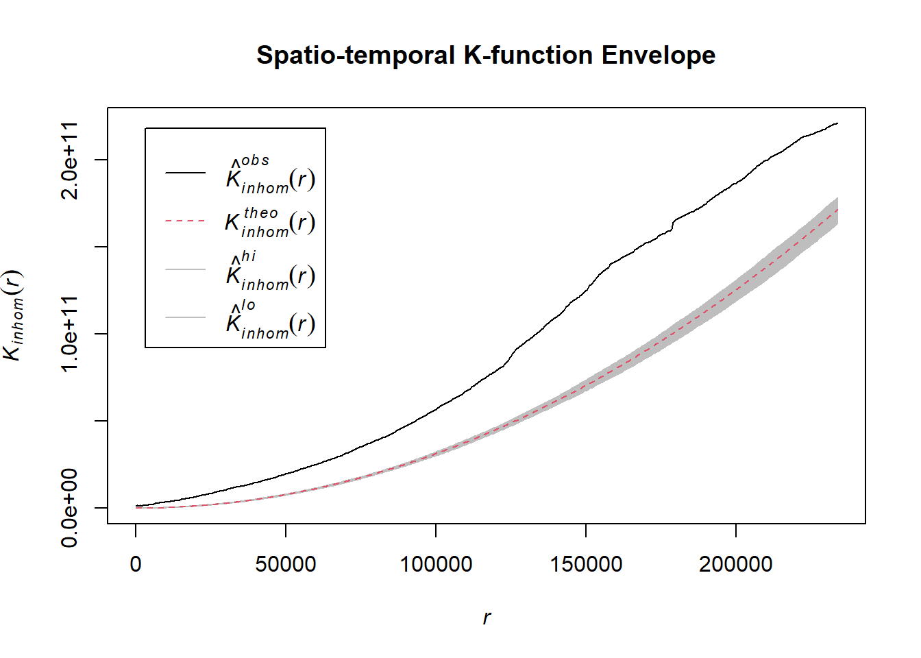
# Assuming `acled_spatio_ppp_owin` is your spatio-temporal point pattern object:
acled_spatio_ppp_owin <- acled_quarters_2023_ppp[regions_owin]
K_st <- Kinhom(acled_spatio_ppp_owin, correction="border")
# Plot the result for visual inspection
plot(K_st, main = "Spatio-temporal K-function", legend=TRUE)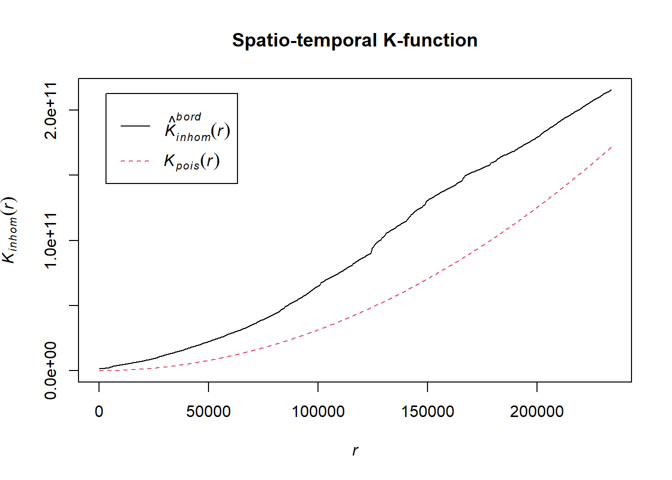
# Perform the CSR test with 99 simulations
K_ck.csr <- envelope(acled_spatio_ppp_owin, Kinhom, nsim=99, correction="border", parallel = parallel::detectCores())Generating 99 simulations of CSR ...
1, 2, [3:37 remaining] 3,
[3:40 remaining] 4, [3:36 remaining] 5, [3:32 remaining] 6,
[3:36 remaining] 7, [3:33 remaining] 8, [3:29 remaining] 9,
[3:25 remaining] 10, [3:28 remaining] 11, [3:25 remaining] 12,
[3:23 remaining] 13, [3:20 remaining] 14, [3:18 remaining] 15,
[3:16 remaining] 16, [3:13 remaining] 17, [3:12 remaining] 18,
[3:09 remaining] 19, [3:08 remaining] 20, [3:06 remaining] 21,
[3:03 remaining] 22, [3:01 remaining] 23, [2:58 remaining] 24,
[2:55 remaining] 25, [2:53 remaining] 26, [2:50 remaining] 27,
[2:48 remaining] 28, [2:45 remaining] 29, [2:43 remaining] 30,
[2:40 remaining] 31, [2:38 remaining] 32, [2:36 remaining] 33,
[2:33 remaining] 34, [2:31 remaining] 35, [2:30 remaining] 36,
[2:28 remaining] 37, [2:26 remaining] 38, [2:23 remaining] 39,
[2:21 remaining] 40, [2:19 remaining] 41, [2:16 remaining] 42,
[2:14 remaining] 43, [2:11 remaining] 44, [2:09 remaining] 45,
[2:07 remaining] 46, [2:04 remaining] 47, [2:02 remaining] 48,
[1:59 remaining] 49, [1:57 remaining] 50, [1:54 remaining] 51,
[1:52 remaining] 52, [1:49 remaining] 53, [1:47 remaining] 54,
[1:45 remaining] 55, [1:42 remaining] 56, [1:40 remaining] 57,
[1:38 remaining] 58, [1:35 remaining] 59, [1:33 remaining] 60,
[1:30 remaining] 61, [1:28 remaining] 62, [1:26 remaining] 63,
[1:24 remaining] 64, [1:21 remaining] 65, [1:19 remaining] 66,
[1:17 remaining] 67, [1:15 remaining] 68, [1:12 remaining] 69,
[1:10 remaining] 70, [1:08 remaining] 71, [1:06 remaining] 72,
[1:04 remaining] 73, [1:02 remaining] 74, [59 sec remaining] 75,
[57 sec remaining] 76, [55 sec remaining] 77, [52 sec remaining] 78,
[50 sec remaining] 79, [48 sec remaining] 80, [45 sec remaining] 81,
[43 sec remaining] 82, [41 sec remaining] 83, [38 sec remaining] 84,
[36 sec remaining] 85, [33 sec remaining] 86, [31 sec remaining] 87,
[29 sec remaining] 88, [26 sec remaining] 89, [24 sec remaining] 90,
[22 sec remaining] 91, [19 sec remaining] 92, [17 sec remaining] 93,
[14 sec remaining] 94, [12 sec remaining] 95, [10 sec remaining] 96,
[7 sec remaining] 97, [5 sec remaining] 98, [2 sec remaining]
99.
Done.# Plot the envelope with the observed K-function
plot(K_ck.csr, main="Spatio-temporal K-function Envelope", legend=TRUE)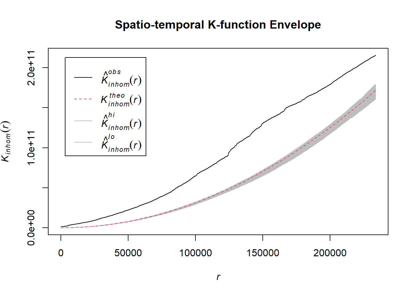
# Assuming `acled_spatio_ppp_owin` is your spatio-temporal point pattern object:
acled_spatio_ppp_owin <- acled_quarters_2024_ppp[regions_owin]
K_st <- Kinhom(acled_spatio_ppp_owin, correction="border")
# Plot the result for visual inspection
plot(K_st, main = "Spatio-temporal K-function", legend=TRUE)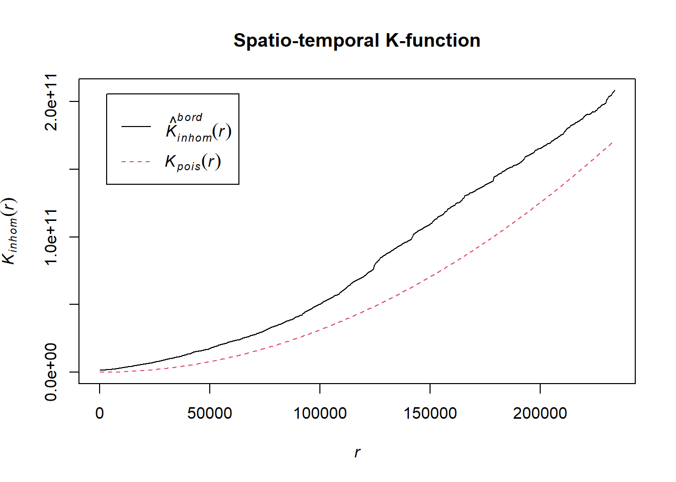
# Perform the CSR test with 99 simulations
K_ck.csr <- envelope(acled_spatio_ppp_owin, Kinhom, nsim=99, correction="border", parallel = parallel::detectCores())Generating 99 simulations of CSR ...
1, 2, 3, 4, 5, 6, 7, 8, 9, 10, 11, 12, 13, 14, 15, 16, 17, 18, 19, 20,
21, 22, 23, 24, 25, 26, 27, 28, 29, 30, 31, 32, 33, 34, 35, 36, 37, 38, 39, 40,
41, 42, 43, 44, 45, 46, 47, 48, 49, 50, 51, 52, 53, 54, 55, 56, 57, 58, 59, 60,
61, 62, 63, 64, 65, 66, 67, 68, 69, 70, 71, 72, 73, 74, 75, 76, 77, 78, 79, 80,
81, 82, 83, 84, 85, 86, 87, 88, 89, 90, 91, 92, 93, 94, 95, 96, 97, 98,
99.
Done.# Plot the envelope with the observed K-function
plot(K_ck.csr, main="Spatio-temporal K-function Envelope", legend=TRUE)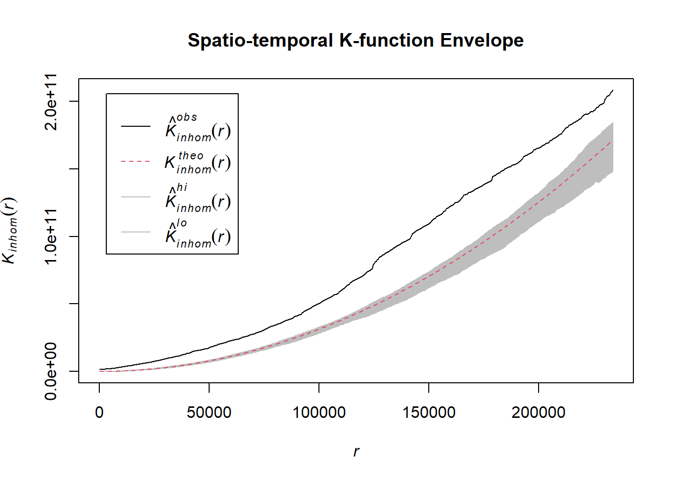
Note
Interpretation: 1. Large Distance Scales: - The x-axis stretches to large distances, and while there is visible divergence between the observed and theoretical K-function, this may reflect clustering at large spatial scales. However, in real-world spatial analyses, large scales may not capture important localized clustering that occurs over smaller distances.
- Envelope Overlap:
- While the black observed curve rises above the simulation envelope, the overall broadness of the envelope may obscure fine distinctions. A closer look at smaller scales or at specific distances would provide a more refined understanding of clustering in specific areas and time periods, particularly for regions like Chin or Mandalay in the context of the Burmese civil war.
- Potential Scale Sensitivity:
- Spatio-temporal processes often show different behaviors at different spatial or temporal scales. While this graph suggests some clustering, it’s possible that examining specific distance ranges more closely (e.g., shorter spatial ranges or focusing on specific temporal windows) could reveal more localized patterns of interaction that are not easily discernible in this large-scale plot.
In conclusion, the general consensus of the plots provides some indication of spatio-temporal clustering, but to gain meaningful insights, a closer, more focused analysis over smaller spatial and temporal distances is required to uncover patterns of conflict that may be masked at these larger scales.
1.8.4 Looking Closer
Visually, we observed that the regions of Chin, Sagaing, Mandalay, and Magway have the highest occurrences of event types such as Explosions/Remote violence, Strategic developments, Battles, and Violence against Civilians. To better understand the spatial and temporal distribution and clustering of these events, we will perform a second-order spatio-temporal point pattern analysis. This will help assess the degree of interaction or clustering of events across space and time within these key regions.
1.8.4.1 Importing the relevant regions into R
chin_sf <- st_read(dsn = "data/chin",
layer = "mmr_chn_polbnda_adm4_mimu_250k")Reading layer `mmr_chn_polbnda_adm4_mimu_250k' from data source
`C:\Users\blzll\OneDrive\Desktop\Y3S1\IS415\Quarto\IS415\Take-home_ex\data\chin'
using driver `ESRI Shapefile'
Simple feature collection with 482 features and 14 fields
Geometry type: POLYGON
Dimension: XY
Bounding box: xmin: 92.6021 ymin: 20.6399 xmax: 94.15303 ymax: 24.10598
Geodetic CRS: WGS 84chin_sf <- st_transform(chin_sf, crs = 32647)chin_owin <- as.owin(chin_sf)magway_sf <- st_read(dsn = "data/sagaing",
layer = "mmr_mgy_polbnda_adm4_wfp_mimu_250k_1")Reading layer `mmr_mgy_polbnda_adm4_wfp_mimu_250k_1' from data source
`C:\Users\blzll\OneDrive\Desktop\Y3S1\IS415\Quarto\IS415\Take-home_ex\data\sagaing'
using driver `ESRI Shapefile'
Simple feature collection with 1599 features and 14 fields
Geometry type: MULTIPOLYGON
Dimension: XY
Bounding box: xmin: 93.84551 ymin: 18.83204 xmax: 95.85919 ymax: 22.77128
Geodetic CRS: WGS 84magway_sf <- st_transform(magway_sf, crs = 32647)magway_owin <- as.owin(magway_sf)mandalay_sf <- st_read(dsn = "data/mandalay",
layer = "mmr_mdy_polbnda_adm4_mimu_250k")Reading layer `mmr_mdy_polbnda_adm4_mimu_250k' from data source
`C:\Users\blzll\OneDrive\Desktop\Y3S1\IS415\Quarto\IS415\Take-home_ex\data\mandalay'
using driver `ESRI Shapefile'
Simple feature collection with 1463 features and 14 fields
Geometry type: MULTIPOLYGON
Dimension: XY
Bounding box: xmin: 94.82973 ymin: 20.19307 xmax: 96.89598 ymax: 23.68381
Geodetic CRS: WGS 84mandalay_sf <- st_transform(mandalay_sf, crs = 32647)mandalay_owin <- as.owin(mandalay_sf)sagaing_sf <- st_read(dsn = "data/magway",
layer = "mmr_sag_polbnda_adm4_250k_mimu_1")Reading layer `mmr_sag_polbnda_adm4_250k_mimu_1' from data source
`C:\Users\blzll\OneDrive\Desktop\Y3S1\IS415\Quarto\IS415\Take-home_ex\data\magway'
using driver `ESRI Shapefile'
Simple feature collection with 1825 features and 14 fields
Geometry type: MULTIPOLYGON
Dimension: XY
Bounding box: xmin: 93.94619 ymin: 21.57594 xmax: 97.0669 ymax: 27.37205
Geodetic CRS: WGS 84sagaing_sf <- st_transform(sagaing_sf, crs = 32647)sagaing_owin <- as.owin(sagaing_sf)temporal_acled_sf <- read_rds("data/rds/temporal_acled_sf.rds")1.8.4.2 Chin Region
# Perform spatial intersection to keep only the points within Chin region
chin_acled_sf <- temporal_acled_sf %>% filter(admin1 == "Chin")
# Plot the Chin region and filtered points
tm_shape(chin_sf) +
tm_polygons() +
tm_shape(chin_acled_sf) +
tm_dots(size = 0.3) +
tm_facets(by = "quarter",
free.coords = FALSE,
drop.units = TRUE) +
tm_layout(main.title = "Region and Boundaries of Chin",
main.title.position = "center",
main.title.size = 1,
legend.outside = TRUE,
frame = TRUE)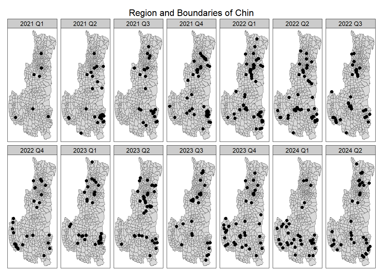
write_rds(chin_acled_sf, "data/rds/chin_acled_sf.rds")1.8.4.2.1 Explosions/Remote violence
Example <- "Explosions/Remote violence"
chin_acled_quarters_2021_ppp <- as.ppp(chin_acled_sf %>%
filter(year == 2021 & event_type == Example) %>%
select(q))
chin_acled_quarters_2022_ppp <- as.ppp(chin_acled_sf %>%
filter(year == 2022 & event_type == Example) %>%
select(q))
chin_acled_quarters_2023_ppp <- as.ppp(chin_acled_sf %>%
filter(year == 2023 & event_type == Example) %>%
select(q))
chin_acled_quarters_2024_ppp <- as.ppp(chin_acled_sf %>%
filter(year == 2024 & event_type == Example) %>%
select(q))# Assuming `acled_spatio_ppp_owin` is your spatio-temporal point pattern object:
acled_spatio_ppp_owin <- chin_acled_quarters_2021_ppp[chin_owin]
K_st <- Kinhom(acled_spatio_ppp_owin, correction="border")
# Plot the result for visual inspection
plot(K_st, main = "Spatio-temporal K-function", legend=TRUE)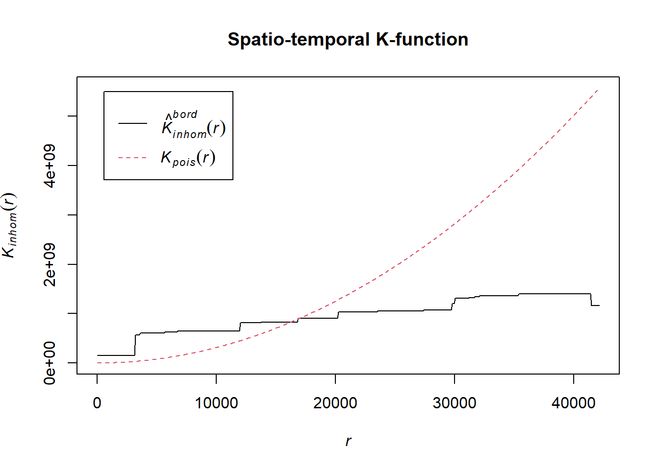
# Perform the CSR test with 99 simulations
K_ck.csr <- envelope(acled_spatio_ppp_owin, Kinhom, nsim=99, correction="border", parallel = parallel::detectCores())Generating 99 simulations of CSR ...
1, 2, 3, 4, 5, 6, 7, 8, 9, 10, 11, 12, 13, 14, 15, 16, 17, 18, 19, 20,
21, 22, 23, 24, 25, 26, 27, 28, 29, 30, 31, 32, 33, 34, 35, 36, 37, 38, 39, 40,
41, 42, 43, 44, 45, 46, 47, 48, 49, 50, 51, 52, 53, 54, 55, 56, 57, 58, 59, 60,
61, 62, 63, 64, 65, 66, 67, 68, 69, 70, 71, 72, 73, 74, 75, 76, 77, 78, 79, 80,
81, 82, 83, 84, 85, 86, 87, 88, 89, 90, 91, 92, 93, 94, 95, 96, 97, 98,
99.
Done.# Plot the envelope with the observed K-function
plot(K_ck.csr, main="Spatio-temporal K-function Envelope", legend=TRUE)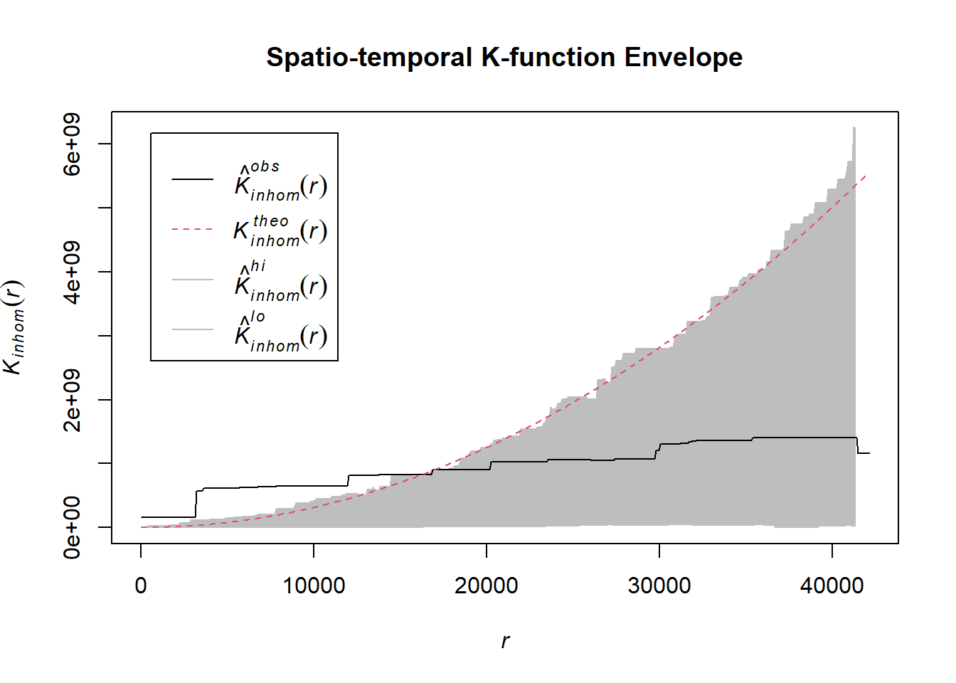
# Assuming `acled_spatio_ppp_owin` is your spatio-temporal point pattern object:
acled_spatio_ppp_owin <- chin_acled_quarters_2022_ppp[chin_owin]
K_st <- Kinhom(acled_spatio_ppp_owin, correction="border")
# Plot the result for visual inspection
plot(K_st, main = "Spatio-temporal K-function", legend=TRUE)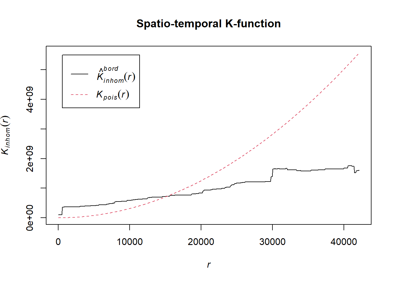
# Perform the CSR test with 99 simulations
K_ck.csr <- envelope(acled_spatio_ppp_owin, Kinhom, nsim=99, correction="border", parallel = parallel::detectCores())Generating 99 simulations of CSR ...
1, 2, 3, 4, 5, 6, 7, 8, 9, 10, 11, 12, 13, 14, 15, 16, 17, 18, 19, 20,
21, 22, 23, 24, 25, 26, 27, 28, 29, 30, 31, 32, 33, 34, 35, 36, 37, 38, 39, 40,
41, 42, 43, 44, 45, 46, 47, 48, 49, 50, 51, 52, 53, 54, 55, 56, 57, 58, 59, 60,
61, 62, 63, 64, 65, 66, 67, 68, 69, 70, 71, 72, 73, 74, 75, 76, 77, 78, 79, 80,
81, 82, 83, 84, 85, 86, 87, 88, 89, 90, 91, 92, 93, 94, 95, 96, 97, 98,
99.
Done.# Plot the envelope with the observed K-function
plot(K_ck.csr, main="Spatio-temporal K-function Envelope", legend=TRUE)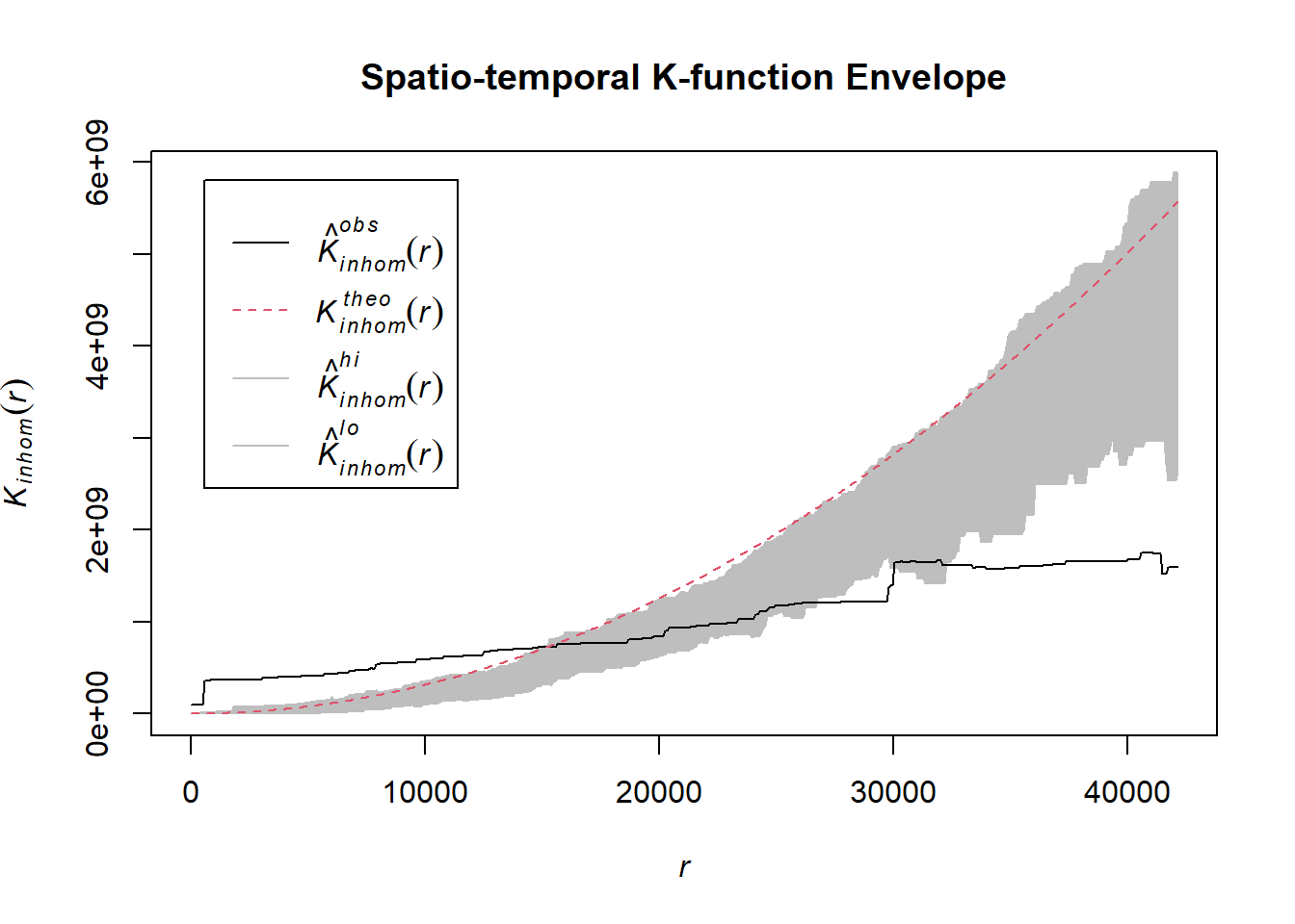
# Assuming `acled_spatio_ppp_owin` is your spatio-temporal point pattern object:
acled_spatio_ppp_owin <- chin_acled_quarters_2023_ppp[chin_owin]
K_st <- Kinhom(acled_spatio_ppp_owin, correction="border")
# Plot the result for visual inspection
plot(K_st, main = "Spatio-temporal K-function", legend=TRUE)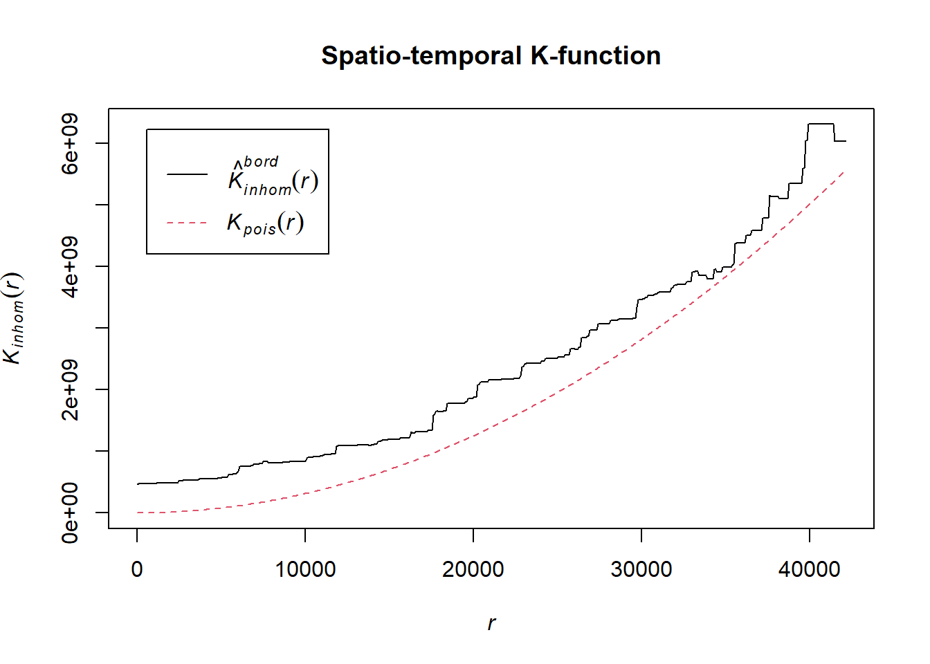
# Perform the CSR test with 99 simulations
K_ck.csr <- envelope(acled_spatio_ppp_owin, Kinhom, nsim=99, correction="border", parallel = parallel::detectCores())Generating 99 simulations of CSR ...
1, 2, 3, 4, 5, 6, 7, 8, 9, 10, 11, 12, 13, 14, 15, 16, 17, 18, 19, 20,
21, 22, 23, 24, 25, 26, 27, 28, 29, 30, 31, 32, 33, 34, 35, 36, 37, 38, 39, 40,
41, 42, 43, 44, 45, 46, 47, 48, 49, 50, 51, 52, 53, 54, 55, 56, 57, 58, 59, 60,
61, 62, 63, 64, 65, 66, 67, 68, 69, 70, 71, 72, 73, 74, 75, 76, 77, 78, 79, 80,
81, 82, 83, 84, 85, 86, 87, 88, 89, 90, 91, 92, 93, 94, 95, 96, 97, 98,
99.
Done.# Plot the envelope with the observed K-function
plot(K_ck.csr, main="Spatio-temporal K-function Envelope", legend=TRUE)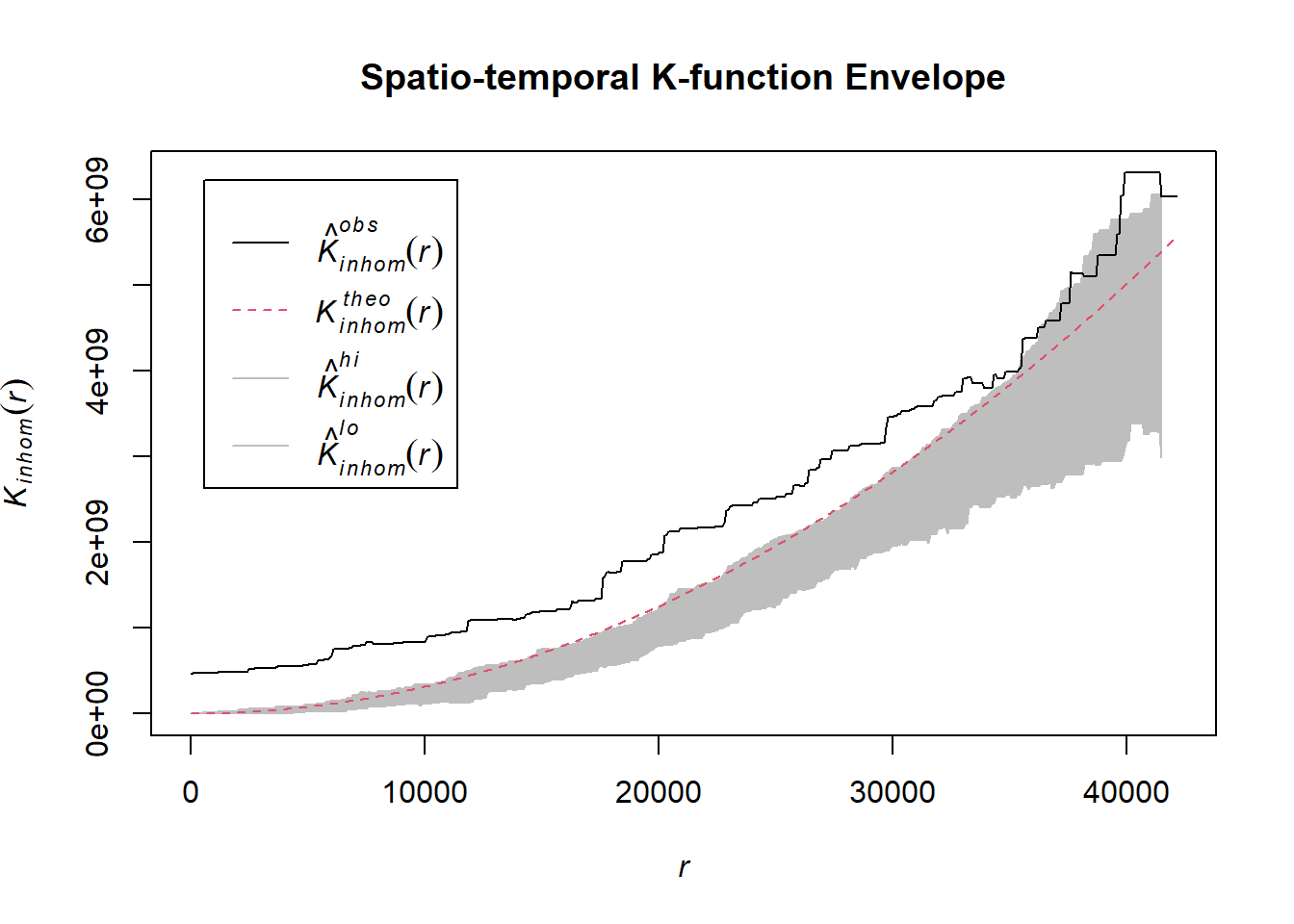
# Assuming `acled_spatio_ppp_owin` is your spatio-temporal point pattern object:
acled_spatio_ppp_owin <- chin_acled_quarters_2024_ppp[chin_owin]
K_st <- Kinhom(acled_spatio_ppp_owin, correction="border")
# Plot the result for visual inspection
plot(K_st, main = "Spatio-temporal K-function", legend=TRUE)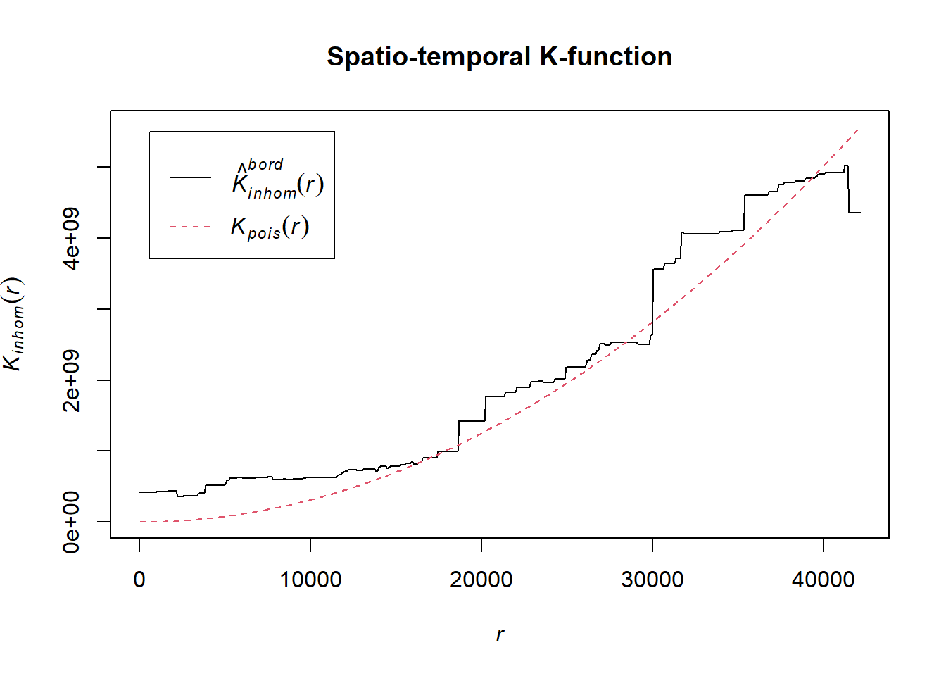
# Perform the CSR test with 99 simulations
K_ck.csr <- envelope(acled_spatio_ppp_owin, Kinhom, nsim=99, correction="border", parallel = parallel::detectCores())Generating 99 simulations of CSR ...
1, 2, 3, 4, 5, 6, 7, 8, 9, 10, 11, 12, 13, 14, 15, 16, 17, 18, 19, 20,
21, 22, 23, 24, 25, 26, 27, 28, 29, 30, 31, 32, 33, 34, 35, 36, 37, 38, 39, 40,
41, 42, 43, 44, 45, 46, 47, 48, 49, 50, 51, 52, 53, 54, 55, 56, 57, 58, 59, 60,
61, 62, 63, 64, 65, 66, 67, 68, 69, 70, 71, 72, 73, 74, 75, 76, 77, 78, 79, 80,
81, 82, 83, 84, 85, 86, 87, 88, 89, 90, 91, 92, 93, 94, 95, 96, 97, 98,
99.
Done.# Plot the envelope with the observed K-function
plot(K_ck.csr, main="Spatio-temporal K-function Envelope", legend=TRUE)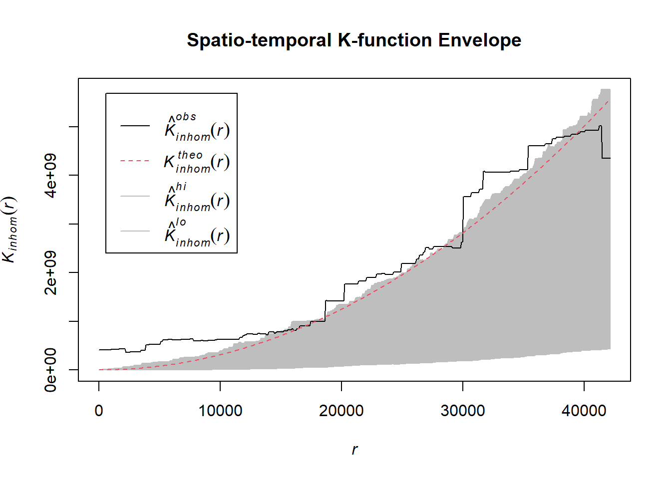
1.8.4.2.2 Strategic developments
Example <- "Strategic developments"
chin_acled_quarters_2021_ppp <- as.ppp(chin_acled_sf %>%
filter(year == 2021 & event_type == Example) %>%
select(q))
chin_acled_quarters_2022_ppp <- as.ppp(chin_acled_sf %>%
filter(year == 2022 & event_type == Example) %>%
select(q))
chin_acled_quarters_2023_ppp <- as.ppp(chin_acled_sf %>%
filter(year == 2023 & event_type == Example) %>%
select(q))
chin_acled_quarters_2024_ppp <- as.ppp(chin_acled_sf %>%
filter(year == 2024 & event_type == Example) %>%
select(q))# Assuming `acled_spatio_ppp_owin` is your spatio-temporal point pattern object:
acled_spatio_ppp_owin <- chin_acled_quarters_2021_ppp[chin_owin]
K_st <- Kinhom(acled_spatio_ppp_owin, correction="border")
# Plot the result for visual inspection
plot(K_st, main = "Spatio-temporal K-function", legend=TRUE)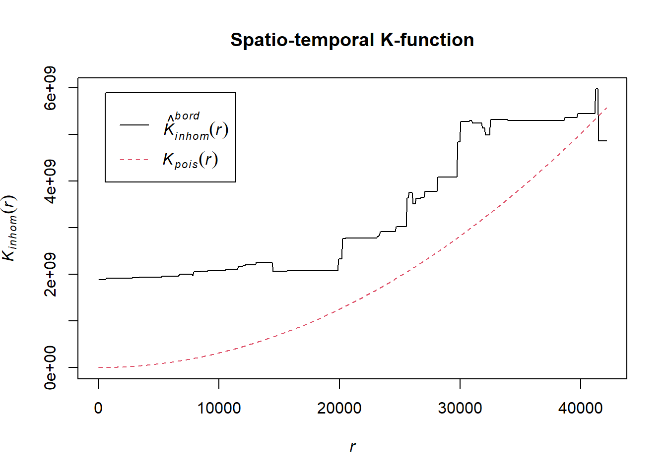
# Perform the CSR test with 99 simulations
K_ck.csr <- envelope(acled_spatio_ppp_owin, Kinhom, nsim=99, correction="border", parallel = parallel::detectCores())Generating 99 simulations of CSR ...
1, 2, 3, 4, 5, 6, 7, 8, 9, 10, 11, 12, 13, 14, 15, 16, 17, 18, 19, 20,
21, 22, 23, 24, 25, 26, 27, 28, 29, 30, 31, 32, 33, 34, 35, 36, 37, 38, 39, 40,
41, 42, 43, 44, 45, 46, 47, 48, 49, 50, 51, 52, 53, 54, 55, 56, 57, 58, 59, 60,
61, 62, 63, 64, 65, 66, 67, 68, 69, 70, 71, 72, 73, 74, 75, 76, 77, 78, 79, 80,
81, 82, 83, 84, 85, 86, 87, 88, 89, 90, 91, 92, 93, 94, 95, 96, 97, 98,
99.
Done.# Plot the envelope with the observed K-function
plot(K_ck.csr, main="Spatio-temporal K-function Envelope", legend=TRUE)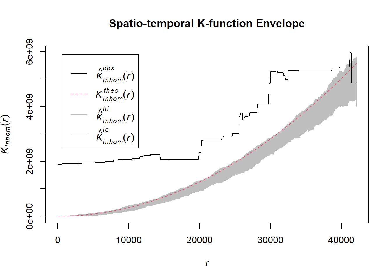
# Assuming `acled_spatio_ppp_owin` is your spatio-temporal point pattern object:
acled_spatio_ppp_owin <- chin_acled_quarters_2022_ppp[chin_owin]
K_st <- Kinhom(acled_spatio_ppp_owin, correction="border")
# Plot the result for visual inspection
plot(K_st, main = "Spatio-temporal K-function", legend=TRUE)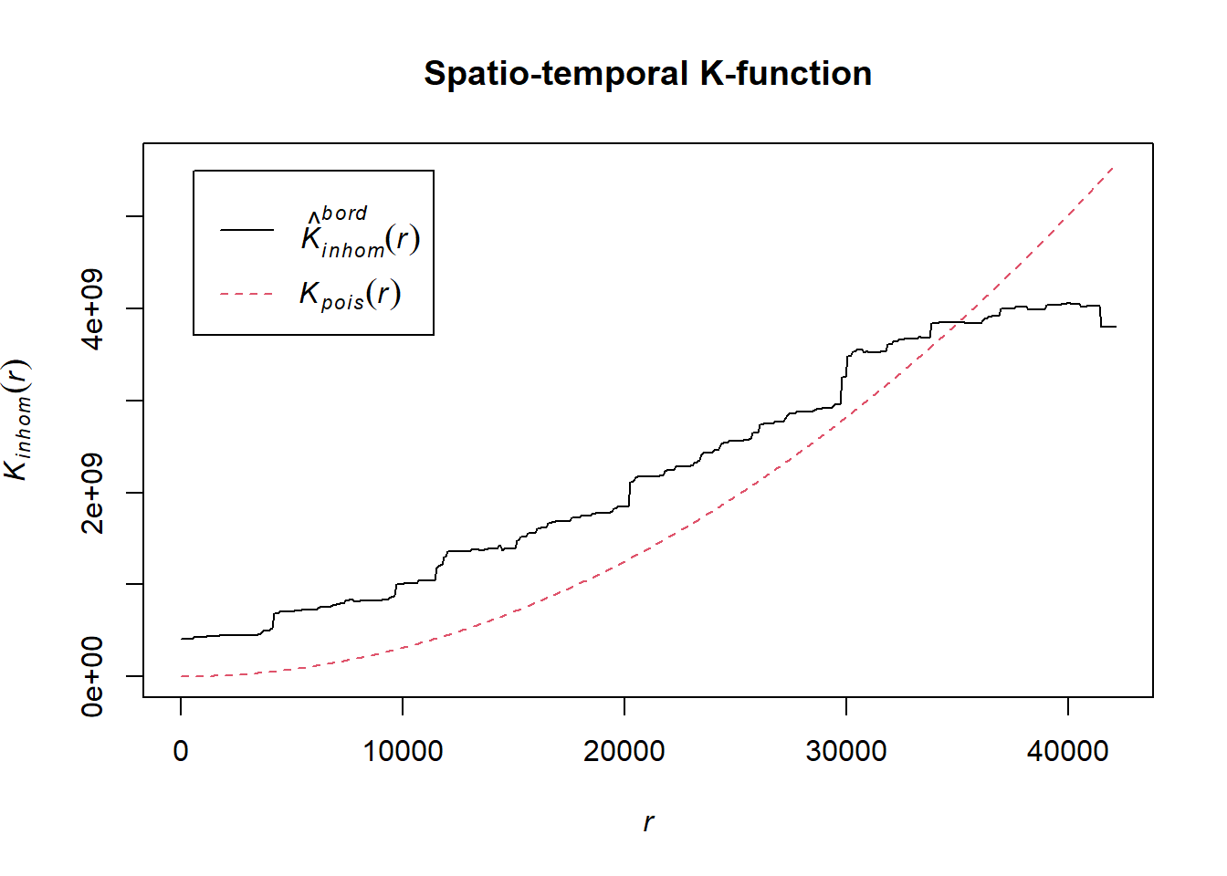
# Perform the CSR test with 99 simulations
K_ck.csr <- envelope(acled_spatio_ppp_owin, Kinhom, nsim=99, correction="border", parallel = parallel::detectCores())Generating 99 simulations of CSR ...
1, 2, 3, 4, 5, 6, 7, 8, 9, 10, 11, 12, 13, 14, 15, 16, 17, 18, 19, 20,
21, 22, 23, 24, 25, 26, 27, 28, 29, 30, 31, 32, 33, 34, 35, 36, 37, 38, 39, 40,
41, 42, 43, 44, 45, 46, 47, 48, 49, 50, 51, 52, 53, 54, 55, 56, 57, 58, 59, 60,
61, 62, 63, 64, 65, 66, 67, 68, 69, 70, 71, 72, 73, 74, 75, 76, 77, 78, 79, 80,
81, 82, 83, 84, 85, 86, 87, 88, 89, 90, 91, 92, 93, 94, 95, 96, 97, 98,
99.
Done.# Plot the envelope with the observed K-function
plot(K_ck.csr, main="Spatio-temporal K-function Envelope", legend=TRUE)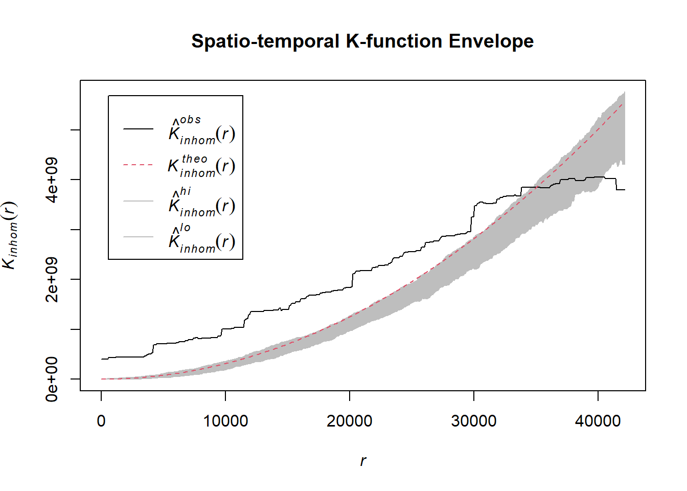
# Assuming `acled_spatio_ppp_owin` is your spatio-temporal point pattern object:
acled_spatio_ppp_owin <- chin_acled_quarters_2023_ppp[chin_owin]
K_st <- Kinhom(acled_spatio_ppp_owin, correction="border")
# Plot the result for visual inspection
plot(K_st, main = "Spatio-temporal K-function", legend=TRUE)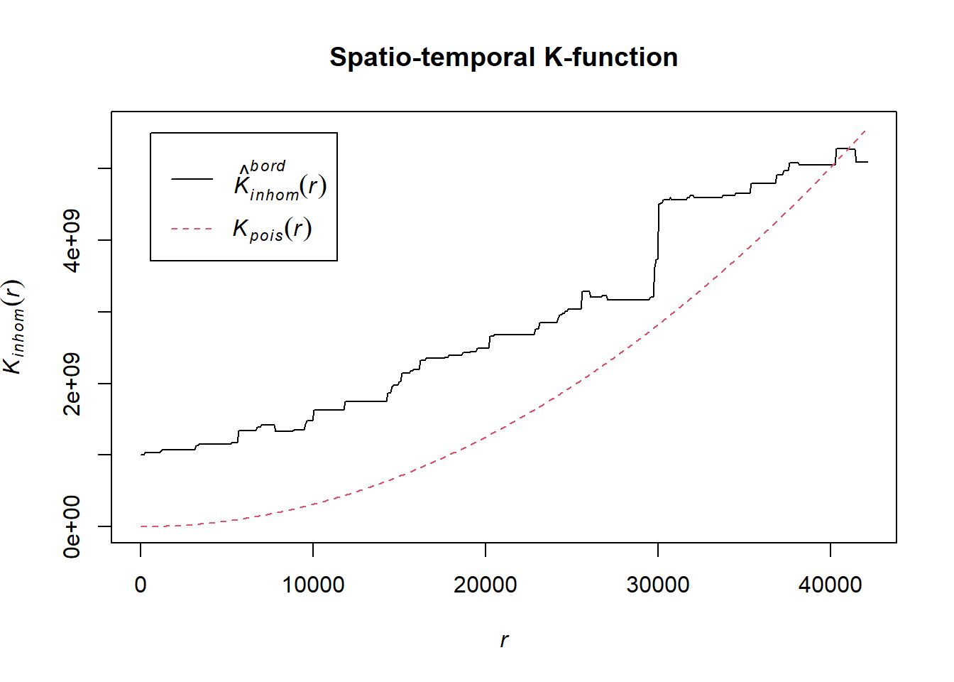
# Perform the CSR test with 99 simulations
K_ck.csr <- envelope(acled_spatio_ppp_owin, Kinhom, nsim=99, correction="border", parallel = parallel::detectCores())Generating 99 simulations of CSR ...
1, 2, 3, 4, 5, 6, 7, 8, 9, 10, 11, 12, 13, 14, 15, 16, 17, 18, 19, 20,
21, 22, 23, 24, 25, 26, 27, 28, 29, 30, 31, 32, 33, 34, 35, 36, 37, 38, 39, 40,
41, 42, 43, 44, 45, 46, 47, 48, 49, 50, 51, 52, 53, 54, 55, 56, 57, 58, 59, 60,
61, 62, 63, 64, 65, 66, 67, 68, 69, 70, 71, 72, 73, 74, 75, 76, 77, 78, 79, 80,
81, 82, 83, 84, 85, 86, 87, 88, 89, 90, 91, 92, 93, 94, 95, 96, 97, 98,
99.
Done.# Plot the envelope with the observed K-function
plot(K_ck.csr, main="Spatio-temporal K-function Envelope", legend=TRUE)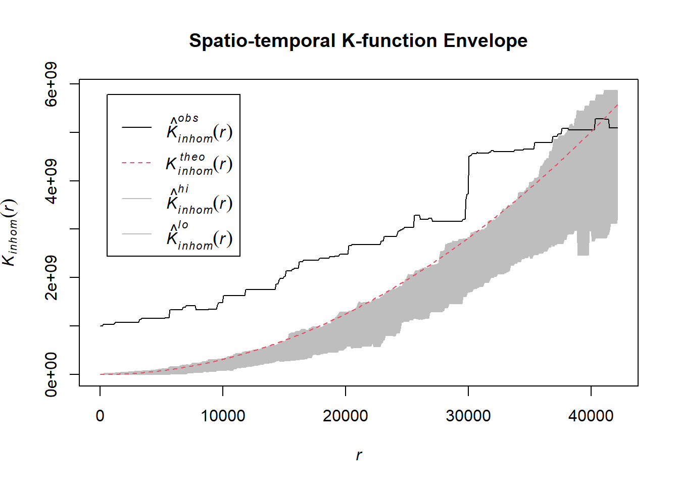
# Assuming `acled_spatio_ppp_owin` is your spatio-temporal point pattern object:
acled_spatio_ppp_owin <- chin_acled_quarters_2024_ppp[chin_owin]
K_st <- Kinhom(acled_spatio_ppp_owin, correction="border")
# Plot the result for visual inspection
plot(K_st, main = "Spatio-temporal K-function", legend=TRUE)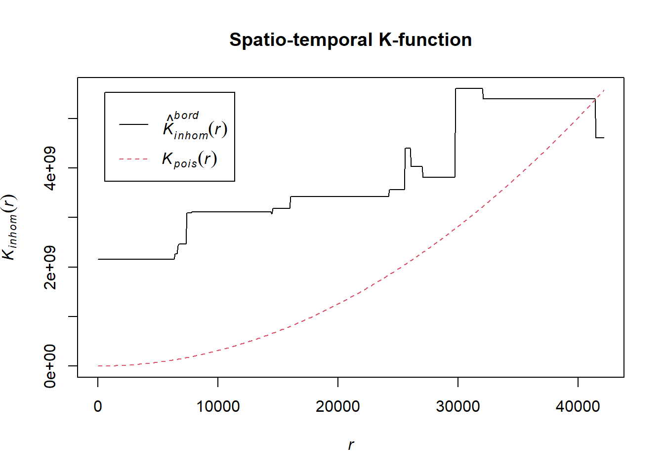
# Perform the CSR test with 99 simulations
K_ck.csr <- envelope(acled_spatio_ppp_owin, Kinhom, nsim=99, correction="border", parallel = parallel::detectCores())Generating 99 simulations of CSR ...
1, 2, 3, 4, 5, 6, 7, 8, 9, 10, 11, 12, 13, 14, 15, 16, 17, 18, 19, 20,
21, 22, 23, 24, 25, 26, 27, 28, 29, 30, 31, 32, 33, 34, 35, 36, 37, 38, 39, 40,
41, 42, 43, 44, 45, 46, 47, 48, 49, 50, 51, 52, 53, 54, 55, 56, 57, 58, 59, 60,
61, 62, 63, 64, 65, 66, 67, 68, 69, 70, 71, 72, 73, 74, 75, 76, 77, 78, 79, 80,
81, 82, 83, 84, 85, 86, 87, 88, 89, 90, 91, 92, 93, 94, 95, 96, 97, 98,
99.
Done.# Plot the envelope with the observed K-function
plot(K_ck.csr, main="Spatio-temporal K-function Envelope", legend=TRUE)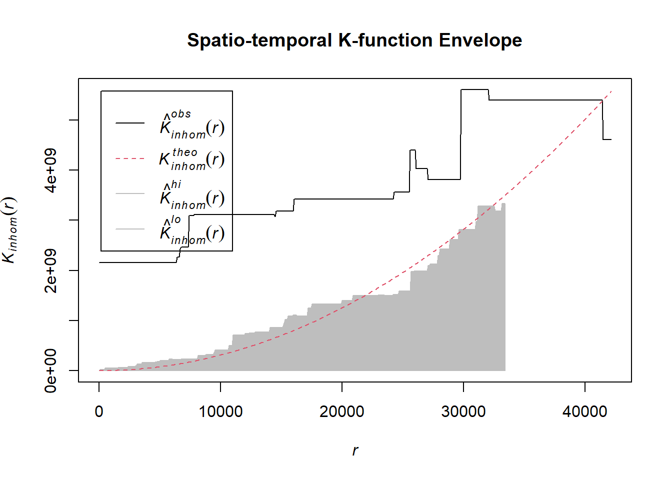
1.8.4.2.3 Battles
Example <- "Battles"
chin_acled_quarters_2021_ppp <- as.ppp(chin_acled_sf %>%
filter(year == 2021 & event_type == Example) %>%
select(q))
chin_acled_quarters_2022_ppp <- as.ppp(chin_acled_sf %>%
filter(year == 2022 & event_type == Example) %>%
select(q))
chin_acled_quarters_2023_ppp <- as.ppp(chin_acled_sf %>%
filter(year == 2023 & event_type == Example) %>%
select(q))
chin_acled_quarters_2024_ppp <- as.ppp(chin_acled_sf %>%
filter(year == 2024 & event_type == Example) %>%
select(q))# Assuming `acled_spatio_ppp_owin` is your spatio-temporal point pattern object:
acled_spatio_ppp_owin <- chin_acled_quarters_2021_ppp[chin_owin]
K_st <- Kinhom(acled_spatio_ppp_owin, correction="border")
# Plot the result for visual inspection
plot(K_st, main = "Spatio-temporal K-function", legend=TRUE)
# Perform the CSR test with 99 simulations
K_ck.csr <- envelope(acled_spatio_ppp_owin, Kinhom, nsim=99, correction="border", parallel = parallel::detectCores())Generating 99 simulations of CSR ...
1, 2, 3, 4, 5, 6, 7, 8, 9, 10, 11, 12, 13, 14, 15, 16, 17, 18, 19, 20,
21, 22, 23, 24, 25, 26, 27, 28, 29, 30, 31, 32, 33, 34, 35, 36, 37, 38, 39, 40,
41, 42, 43, 44, 45, 46, 47, 48, 49, 50, 51, 52, 53, 54, 55, 56, 57, 58, 59, 60,
61, 62, 63, 64, 65, 66, 67, 68, 69, 70, 71, 72, 73, 74, 75, 76, 77, 78, 79, 80,
81, 82, 83, 84, 85, 86, 87, 88, 89, 90, 91, 92, 93, 94, 95, 96, 97, 98,
99.
Done.# Plot the envelope with the observed K-function
plot(K_ck.csr, main="Spatio-temporal K-function Envelope", legend=TRUE)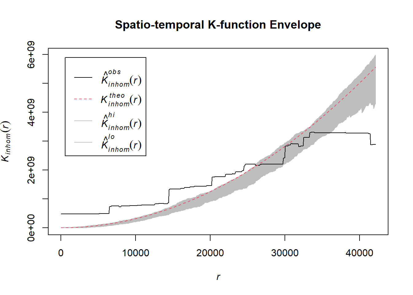
# Assuming `acled_spatio_ppp_owin` is your spatio-temporal point pattern object:
acled_spatio_ppp_owin <- chin_acled_quarters_2022_ppp[chin_owin]
K_st <- Kinhom(acled_spatio_ppp_owin, correction="border")
# Plot the result for visual inspection
plot(K_st, main = "Spatio-temporal K-function", legend=TRUE)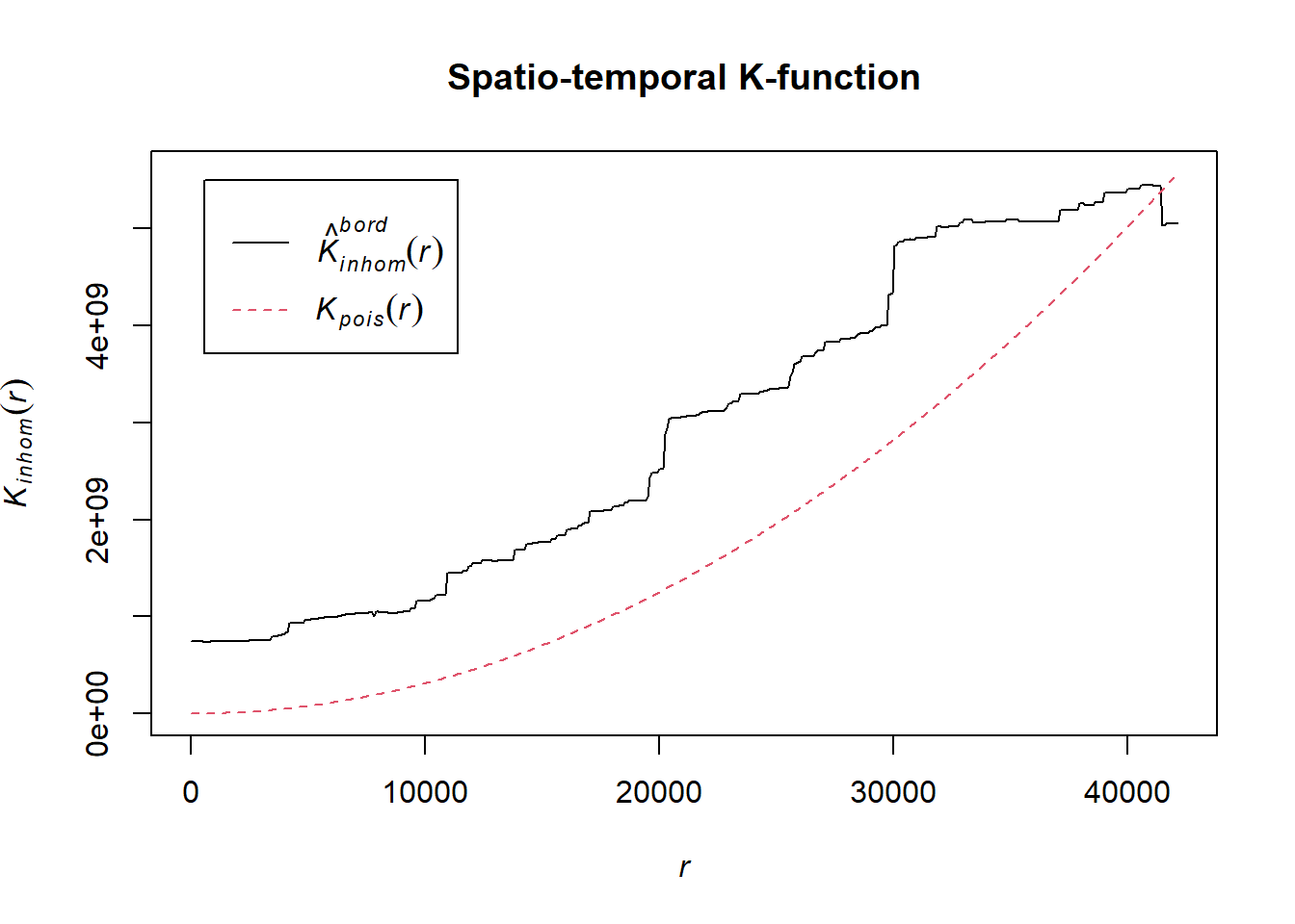
# Perform the CSR test with 99 simulations
K_ck.csr <- envelope(acled_spatio_ppp_owin, Kinhom, nsim=99, correction="border", parallel = parallel::detectCores())Generating 99 simulations of CSR ...
1, 2, 3, 4, 5, 6, 7, 8, 9, 10, 11, 12, 13, 14, 15, 16, 17, 18, 19, 20,
21, 22, 23, 24, 25, 26, 27, 28, 29, 30, 31, 32, 33, 34, 35, 36, 37, 38, 39, 40,
41, 42, 43, 44, 45, 46, 47, 48, 49, 50, 51, 52, 53, 54, 55, 56, 57, 58, 59, 60,
61, 62, 63, 64, 65, 66, 67, 68, 69, 70, 71, 72, 73, 74, 75, 76, 77, 78, 79, 80,
81, 82, 83, 84, 85, 86, 87, 88, 89, 90, 91, 92, 93, 94, 95, 96, 97, 98,
99.
Done.# Plot the envelope with the observed K-function
plot(K_ck.csr, main="Spatio-temporal K-function Envelope", legend=TRUE)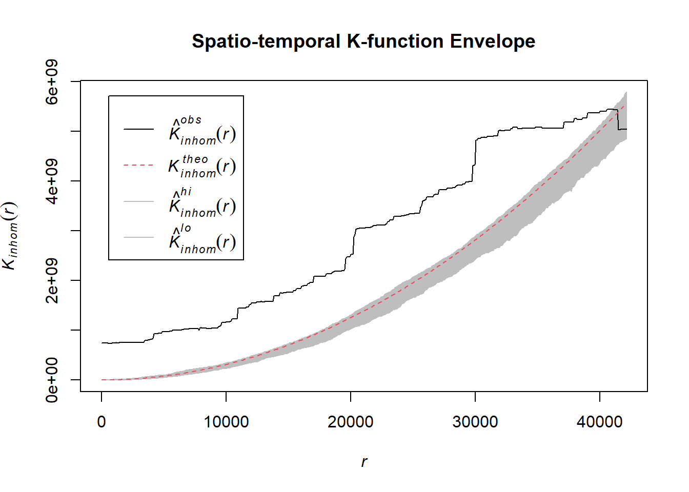
# Assuming `acled_spatio_ppp_owin` is your spatio-temporal point pattern object:
acled_spatio_ppp_owin <- chin_acled_quarters_2023_ppp[chin_owin]
K_st <- Kinhom(acled_spatio_ppp_owin, correction="border")
# Plot the result for visual inspection
plot(K_st, main = "Spatio-temporal K-function", legend=TRUE)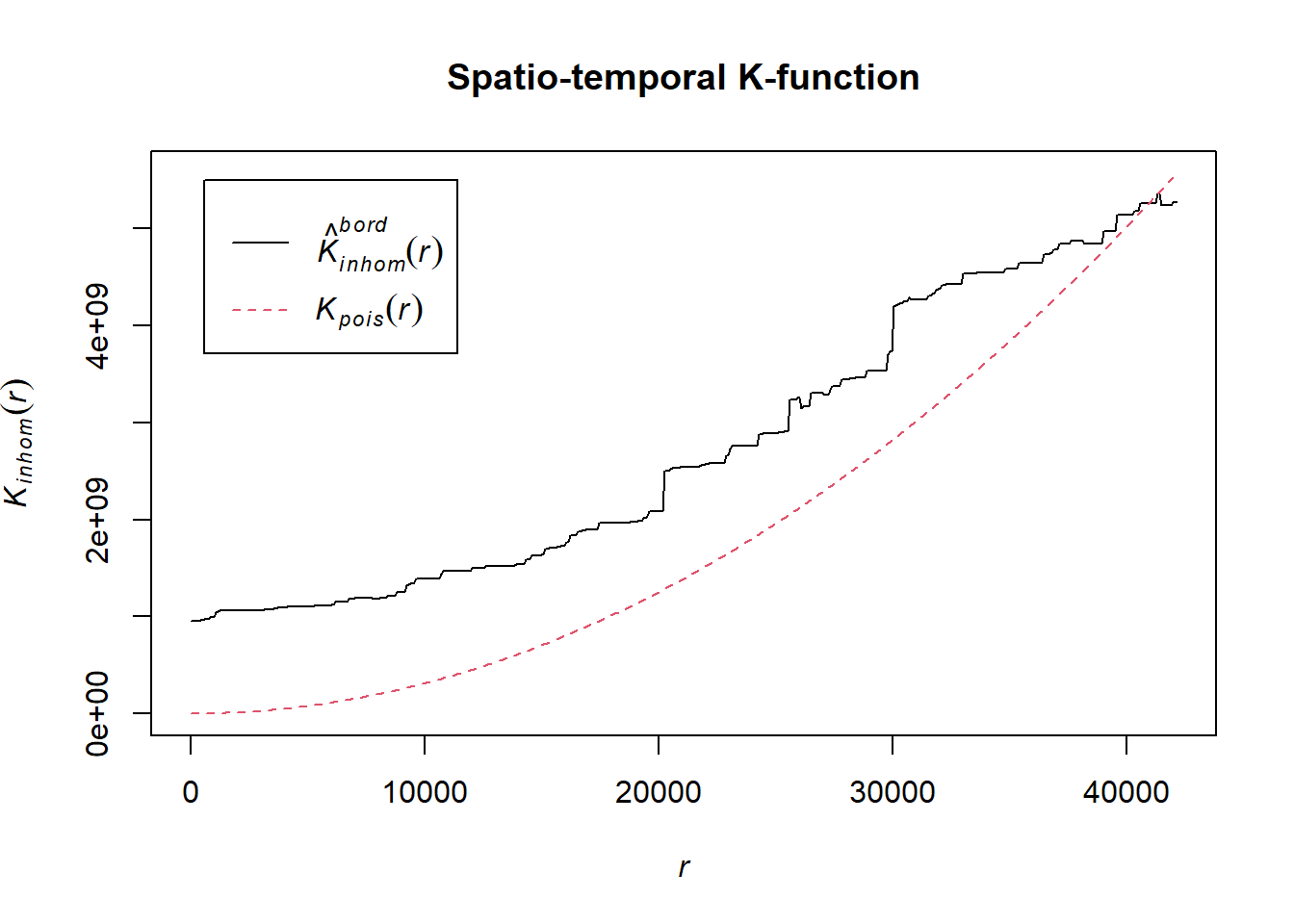
# Perform the CSR test with 99 simulations
K_ck.csr <- envelope(acled_spatio_ppp_owin, Kinhom, nsim=99, correction="border", parallel = parallel::detectCores())Generating 99 simulations of CSR ...
1, 2, 3, 4, 5, 6, 7, 8, 9, 10, 11, 12, 13, 14, 15, 16, 17, 18, 19, 20,
21, 22, 23, 24, 25, 26, 27, 28, 29, 30, 31, 32, 33, 34, 35, 36, 37, 38, 39, 40,
41, 42, 43, 44, 45, 46, 47, 48, 49, 50, 51, 52, 53, 54, 55, 56, 57, 58, 59, 60,
61, 62, 63, 64, 65, 66, 67, 68, 69, 70, 71, 72, 73, 74, 75, 76, 77, 78, 79, 80,
81, 82, 83, 84, 85, 86, 87, 88, 89, 90, 91, 92, 93, 94, 95, 96, 97, 98,
99.
Done.# Plot the envelope with the observed K-function
plot(K_ck.csr, main="Spatio-temporal K-function Envelope", legend=TRUE)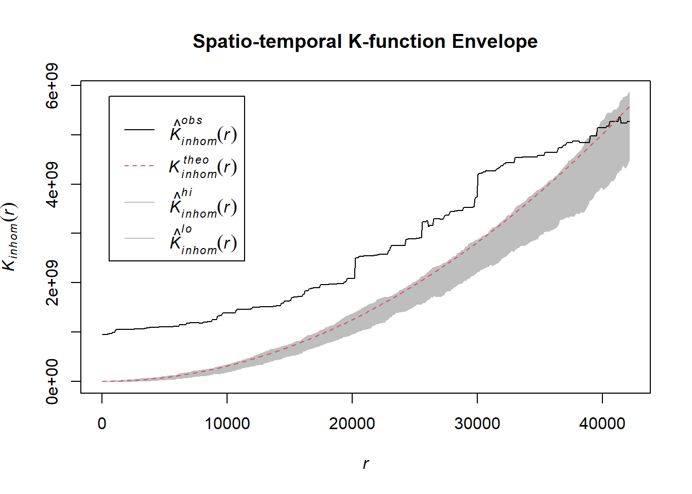
# Assuming `acled_spatio_ppp_owin` is your spatio-temporal point pattern object:
acled_spatio_ppp_owin <- chin_acled_quarters_2024_ppp[chin_owin]
K_st <- Kinhom(acled_spatio_ppp_owin, correction="border")
# Plot the result for visual inspection
plot(K_st, main = "Spatio-temporal K-function", legend=TRUE)
# Perform the CSR test with 99 simulations
K_ck.csr <- envelope(acled_spatio_ppp_owin, Kinhom, nsim=99, correction="border", parallel = parallel::detectCores())Generating 99 simulations of CSR ...
1, 2, 3, 4, 5, 6, 7, 8, 9, 10, 11, 12, 13, 14, 15, 16, 17, 18, 19, 20,
21, 22, 23, 24, 25, 26, 27, 28, 29, 30, 31, 32, 33, 34, 35, 36, 37, 38, 39, 40,
41, 42, 43, 44, 45, 46, 47, 48, 49, 50, 51, 52, 53, 54, 55, 56, 57, 58, 59, 60,
61, 62, 63, 64, 65, 66, 67, 68, 69, 70, 71, 72, 73, 74, 75, 76, 77, 78, 79, 80,
81, 82, 83, 84, 85, 86, 87, 88, 89, 90, 91, 92, 93, 94, 95, 96, 97, 98,
99.
Done.# Plot the envelope with the observed K-function
plot(K_ck.csr, main="Spatio-temporal K-function Envelope", legend=TRUE)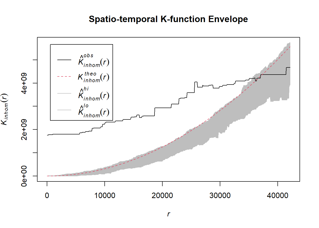
1.8.4.2.4 Violence against civilians
Example <- "Violence against civilians"
acled_quarters_2021_ppp <- as.ppp(temporal_acled_sf %>%
filter(year == 2021 & event_type == Example) %>%
select(q))
acled_quarters_2022_ppp <- as.ppp(temporal_acled_sf %>%
filter(year == 2022 & event_type == Example) %>%
select(q))
acled_quarters_2023_ppp <- as.ppp(temporal_acled_sf %>%
filter(year == 2023 & event_type == Example) %>%
select(q))
acled_quarters_2024_ppp <- as.ppp(temporal_acled_sf %>%
filter(year == 2024 & event_type == Example) %>%
select(q))# Assuming `acled_spatio_ppp_owin` is your spatio-temporal point pattern object:
acled_spatio_ppp_owin <- chin_acled_quarters_2021_ppp[chin_owin]
K_st <- Kinhom(acled_spatio_ppp_owin, correction="border")
# Plot the result for visual inspection
plot(K_st, main = "Spatio-temporal K-function", legend=TRUE)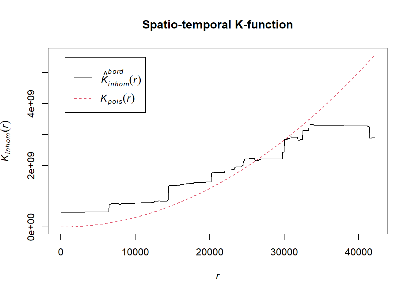
# Perform the CSR test with 99 simulations
K_ck.csr <- envelope(acled_spatio_ppp_owin, Kinhom, nsim=99, correction="border", parallel = parallel::detectCores())Generating 99 simulations of CSR ...
1, 2, 3, 4, 5, 6, 7, 8, 9, 10, 11, 12, 13, 14, 15, 16, 17, 18, 19, 20,
21, 22, 23, 24, 25, 26, 27, 28, 29, 30, 31, 32, 33, 34, 35, 36, 37, 38, 39, 40,
41, 42, 43, 44, 45, 46, 47, 48, 49, 50, 51, 52, 53, 54, 55, 56, 57, 58, 59, 60,
61, 62, 63, 64, 65, 66, 67, 68, 69, 70, 71, 72, 73, 74, 75, 76, 77, 78, 79, 80,
81, 82, 83, 84, 85, 86, 87, 88, 89, 90, 91, 92, 93, 94, 95, 96, 97, 98,
99.
Done.# Plot the envelope with the observed K-function
plot(K_ck.csr, main="Spatio-temporal K-function Envelope", legend=TRUE)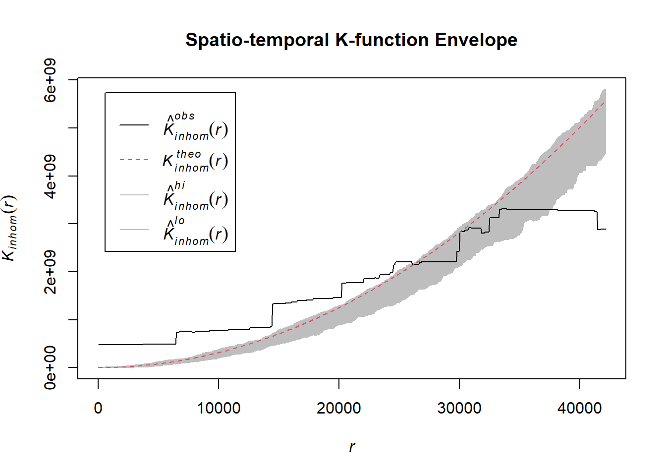
# Assuming `acled_spatio_ppp_owin` is your spatio-temporal point pattern object:
acled_spatio_ppp_owin <- chin_acled_quarters_2022_ppp[chin_owin]
K_st <- Kinhom(acled_spatio_ppp_owin, correction="border")
# Plot the result for visual inspection
plot(K_st, main = "Spatio-temporal K-function", legend=TRUE)
# Perform the CSR test with 99 simulations
K_ck.csr <- envelope(acled_spatio_ppp_owin, Kinhom, nsim=99, correction="border", parallel = parallel::detectCores())Generating 99 simulations of CSR ...
1, 2, 3, 4, 5, 6, 7, 8, 9, 10, 11, 12, 13, 14, 15, 16, 17, 18, 19, 20,
21, 22, 23, 24, 25, 26, 27, 28, 29, 30, 31, 32, 33, 34, 35, 36, 37, 38, 39, 40,
41, 42, 43, 44, 45, 46, 47, 48, 49, 50, 51, 52, 53, 54, 55, 56, 57, 58, 59, 60,
61, 62, 63, 64, 65, 66, 67, 68, 69, 70, 71, 72, 73, 74, 75, 76, 77, 78, 79, 80,
81, 82, 83, 84, 85, 86, 87, 88, 89, 90, 91, 92, 93, 94, 95, 96, 97, 98,
99.
Done.# Plot the envelope with the observed K-function
plot(K_ck.csr, main="Spatio-temporal K-function Envelope", legend=TRUE)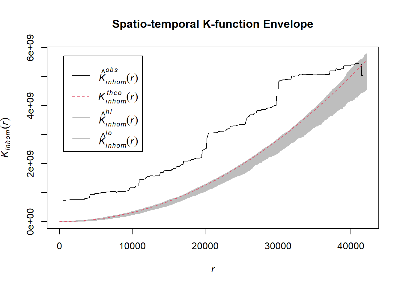
# Assuming `acled_spatio_ppp_owin` is your spatio-temporal point pattern object:
acled_spatio_ppp_owin <- chin_acled_quarters_2023_ppp[chin_owin]
K_st <- Kinhom(acled_spatio_ppp_owin, correction="border")
# Plot the result for visual inspection
plot(K_st, main = "Spatio-temporal K-function", legend=TRUE)
# Perform the CSR test with 99 simulations
K_ck.csr <- envelope(acled_spatio_ppp_owin, Kinhom, nsim=99, correction="border", parallel = parallel::detectCores())Generating 99 simulations of CSR ...
1, 2, 3, 4, 5, 6, 7, 8, 9, 10, 11, 12, 13, 14, 15, 16, 17, 18, 19, 20,
21, 22, 23, 24, 25, 26, 27, 28, 29, 30, 31, 32, 33, 34, 35, 36, 37, 38, 39, 40,
41, 42, 43, 44, 45, 46, 47, 48, 49, 50, 51, 52, 53, 54, 55, 56, 57, 58, 59, 60,
61, 62, 63, 64, 65, 66, 67, 68, 69, 70, 71, 72, 73, 74, 75, 76, 77, 78, 79, 80,
81, 82, 83, 84, 85, 86, 87, 88, 89, 90, 91, 92, 93, 94, 95, 96, 97, 98,
99.
Done.# Plot the envelope with the observed K-function
plot(K_ck.csr, main="Spatio-temporal K-function Envelope", legend=TRUE)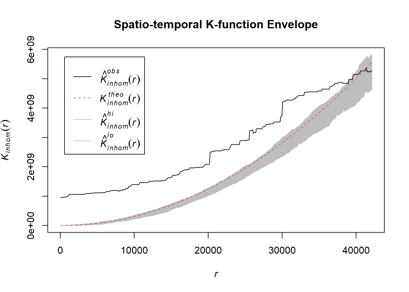
# Assuming `acled_spatio_ppp_owin` is your spatio-temporal point pattern object:
acled_spatio_ppp_owin <- chin_acled_quarters_2024_ppp[chin_owin]
K_st <- Kinhom(acled_spatio_ppp_owin, correction="border")
# Plot the result for visual inspection
plot(K_st, main = "Spatio-temporal K-function", legend=TRUE)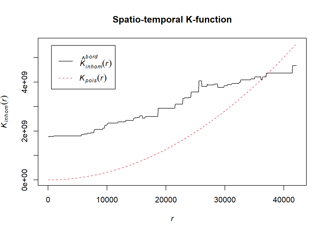
# Perform the CSR test with 99 simulations
K_ck.csr <- envelope(acled_spatio_ppp_owin, Kinhom, nsim=99, correction="border", parallel = parallel::detectCores())Generating 99 simulations of CSR ...
1, 2, 3, 4, 5, 6, 7, 8, 9, 10, 11, 12, 13, 14, 15, 16, 17, 18, 19, 20,
21, 22, 23, 24, 25, 26, 27, 28, 29, 30, 31, 32, 33, 34, 35, 36, 37, 38, 39, 40,
41, 42, 43, 44, 45, 46, 47, 48, 49, 50, 51, 52, 53, 54, 55, 56, 57, 58, 59, 60,
61, 62, 63, 64, 65, 66, 67, 68, 69, 70, 71, 72, 73, 74, 75, 76, 77, 78, 79, 80,
81, 82, 83, 84, 85, 86, 87, 88, 89, 90, 91, 92, 93, 94, 95, 96, 97, 98,
99.
Done.# Plot the envelope with the observed K-function
plot(K_ck.csr, main="Spatio-temporal K-function Envelope", legend=TRUE)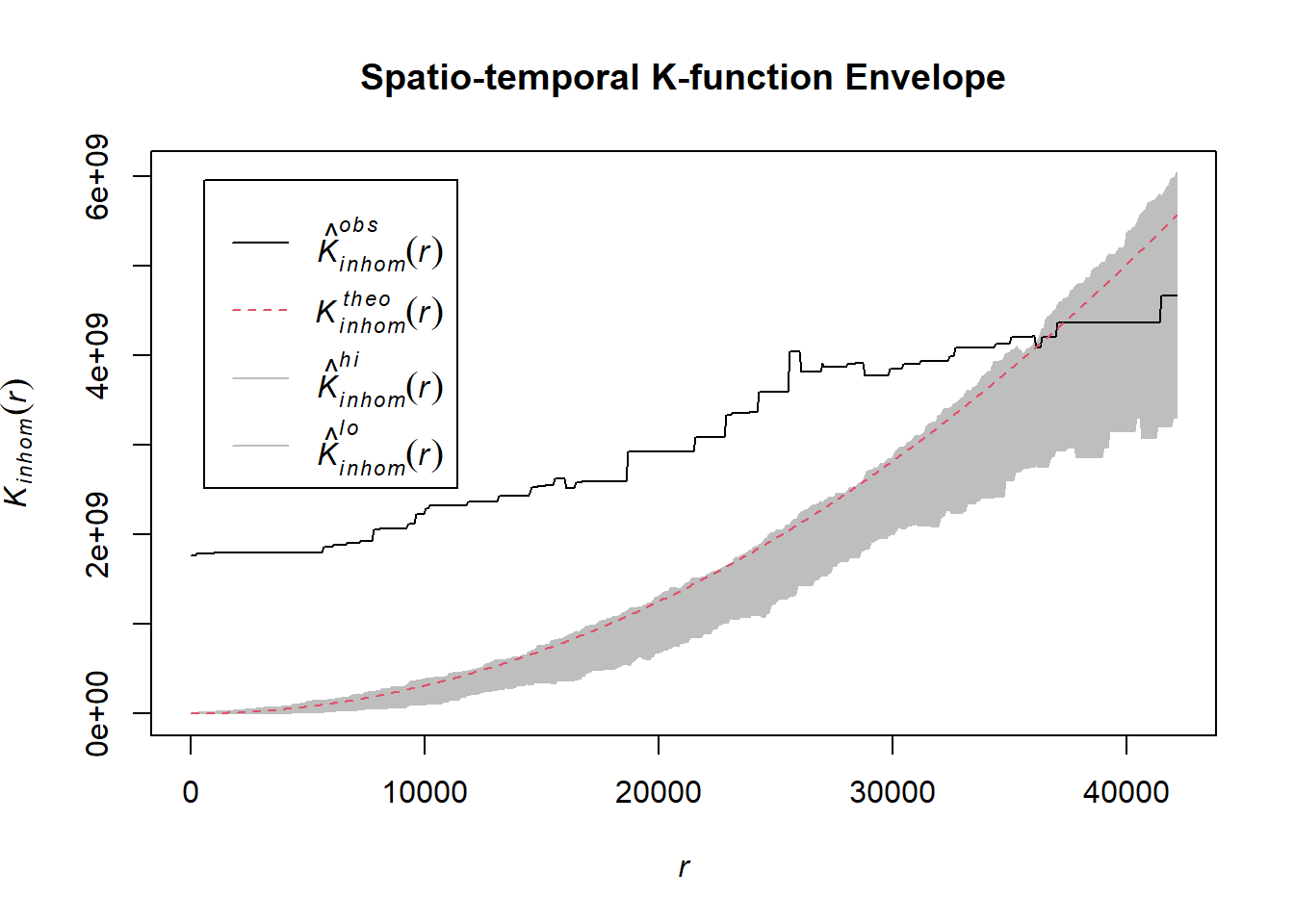
1.8.4.3 Sagaing Region
sagaing_acled_sf <- temporal_acled_sf %>% filter(admin1 == "Sagaing")
tm_shape(sagaing_sf)+
tm_polygons() +
tm_shape(sagaing_acled_sf) +
tm_dots(size=0.1) +
tm_facets(by="quarter",
free.coords=FALSE,
drop.units = TRUE) +
tm_layout(main.title = "Region and Boundaries of Sagaing",
main.title.position = "center",
main.title.size = 1,
legend.outside = TRUE,
frame = TRUE)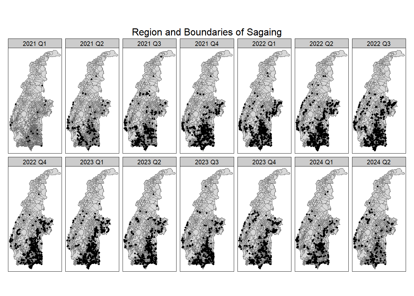
write_rds(sagaing_acled_sf, "data/rds/sagaing_acled_sf.rds")1.8.4.3.1 Explosions/Remote violence
Example <- "Explosions/Remote violence"
sagaing_acled_quarters_2021_ppp <- as.ppp(sagaing_acled_sf %>%
filter(year == 2021 & event_type == Example) %>%
select(q))
sagaing_acled_quarters_2022_ppp <- as.ppp(sagaing_acled_sf %>%
filter(year == 2022 & event_type == Example) %>%
select(q))
sagaing_acled_quarters_2023_ppp <- as.ppp(sagaing_acled_sf %>%
filter(year == 2023 & event_type == Example) %>%
select(q))
sagaing_acled_quarters_2024_ppp <- as.ppp(sagaing_acled_sf %>%
filter(year == 2024 & event_type == Example) %>%
select(q))# Assuming `acled_spatio_ppp_owin` is your spatio-temporal point pattern object:
acled_spatio_ppp_owin <- sagaing_acled_quarters_2021_ppp[sagaing_owin]
K_st <- Kinhom(acled_spatio_ppp_owin, correction="border")
# Plot the result for visual inspection
plot(K_st, main = "Spatio-temporal K-function", legend=TRUE)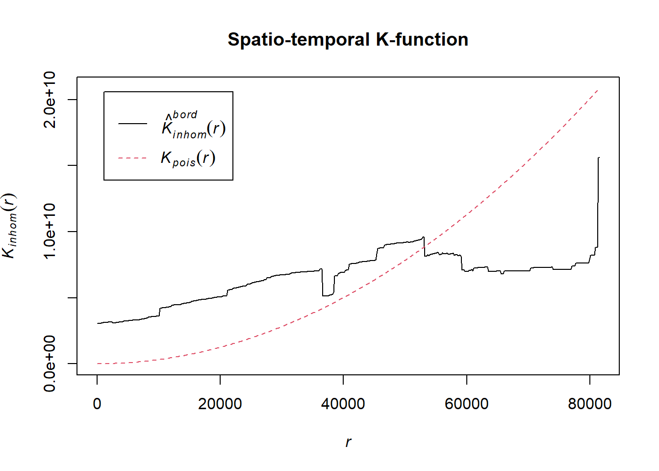
# Perform the CSR test with 99 simulations
K_ck.csr <- envelope(acled_spatio_ppp_owin, Kinhom, nsim=99, correction="border", parallel = parallel::detectCores())Generating 99 simulations of CSR ...
1, 2, 3, 4, 5, 6, 7, 8, 9, 10, 11, 12, 13, 14, 15, 16, 17, 18, 19, 20,
21, 22, 23, 24, 25, 26, 27, 28, 29, 30, 31, 32, 33, 34, 35, 36, 37, 38, 39, 40,
41, 42, 43, 44, 45, 46, 47, 48, 49, 50, 51, 52, 53, 54, 55, 56, 57, 58, 59, 60,
61, 62, 63, 64, 65, 66, 67, 68, 69, 70, 71, 72, 73, 74, 75, 76, 77, 78, 79, 80,
81, 82, 83, 84, 85, 86, 87, 88, 89, 90, 91, 92, 93, 94, 95, 96, 97, 98,
99.
Done.# Plot the envelope with the observed K-function
plot(K_ck.csr, main="Spatio-temporal K-function Envelope", legend=TRUE)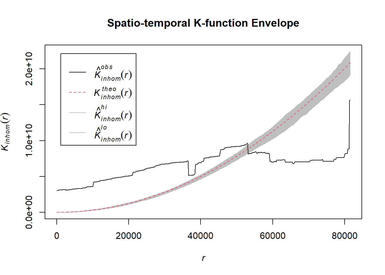
# Assuming `acled_spatio_ppp_owin` is your spatio-temporal point pattern object:
acled_spatio_ppp_owin <- sagaing_acled_quarters_2022_ppp[sagaing_owin]
K_st <- Kinhom(acled_spatio_ppp_owin, correction="border")
# Plot the result for visual inspection
plot(K_st, main = "Spatio-temporal K-function", legend=TRUE)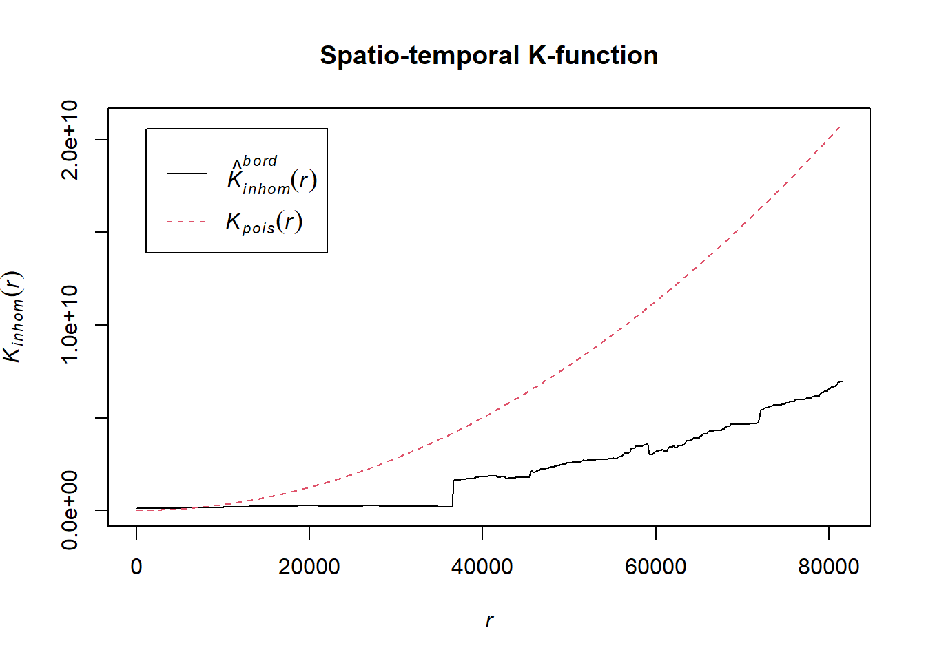
# Perform the CSR test with 99 simulations
K_ck.csr <- envelope(acled_spatio_ppp_owin, Kinhom, nsim=99, correction="border", parallel = parallel::detectCores())Generating 99 simulations of CSR ...
1, 2, 3, 4, 5, 6, 7, 8, 9, 10, 11, 12, 13, 14, 15, 16, 17, 18, 19, 20,
21, 22, 23, 24, 25, 26, 27, 28, 29, 30, 31, 32, 33, 34, 35, 36, 37, 38, 39, 40,
41, 42, 43, 44, 45, 46, 47, 48, 49, 50, 51, 52, 53, 54, 55, 56, 57, 58, 59, 60,
61, 62, 63, 64, 65, 66, 67, 68, 69, 70, 71, 72, 73, 74, 75, 76, 77, 78, 79, 80,
81, 82, 83, 84, 85, 86, 87, 88, 89, 90, 91, 92, 93, 94, 95, 96, 97, 98,
99.
Done.# Plot the envelope with the observed K-function
plot(K_ck.csr, main="Spatio-temporal K-function Envelope", legend=TRUE)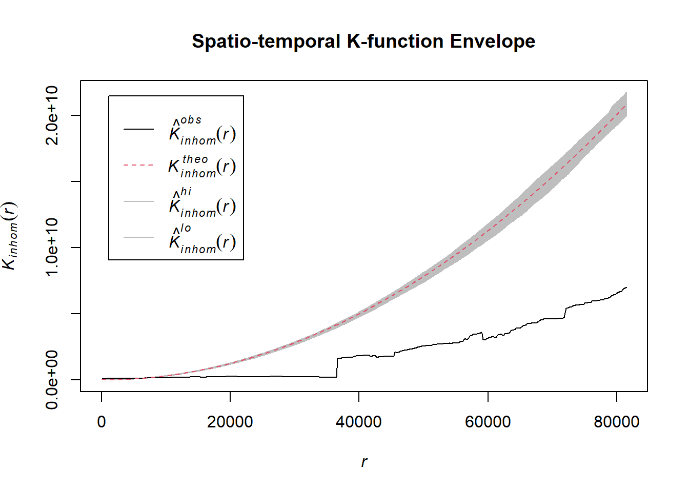
# Assuming `acled_spatio_ppp_owin` is your spatio-temporal point pattern object:
acled_spatio_ppp_owin <- sagaing_acled_quarters_2023_ppp[sagaing_owin]
K_st <- Kinhom(acled_spatio_ppp_owin, correction="border")
# Plot the result for visual inspection
plot(K_st, main = "Spatio-temporal K-function", legend=TRUE)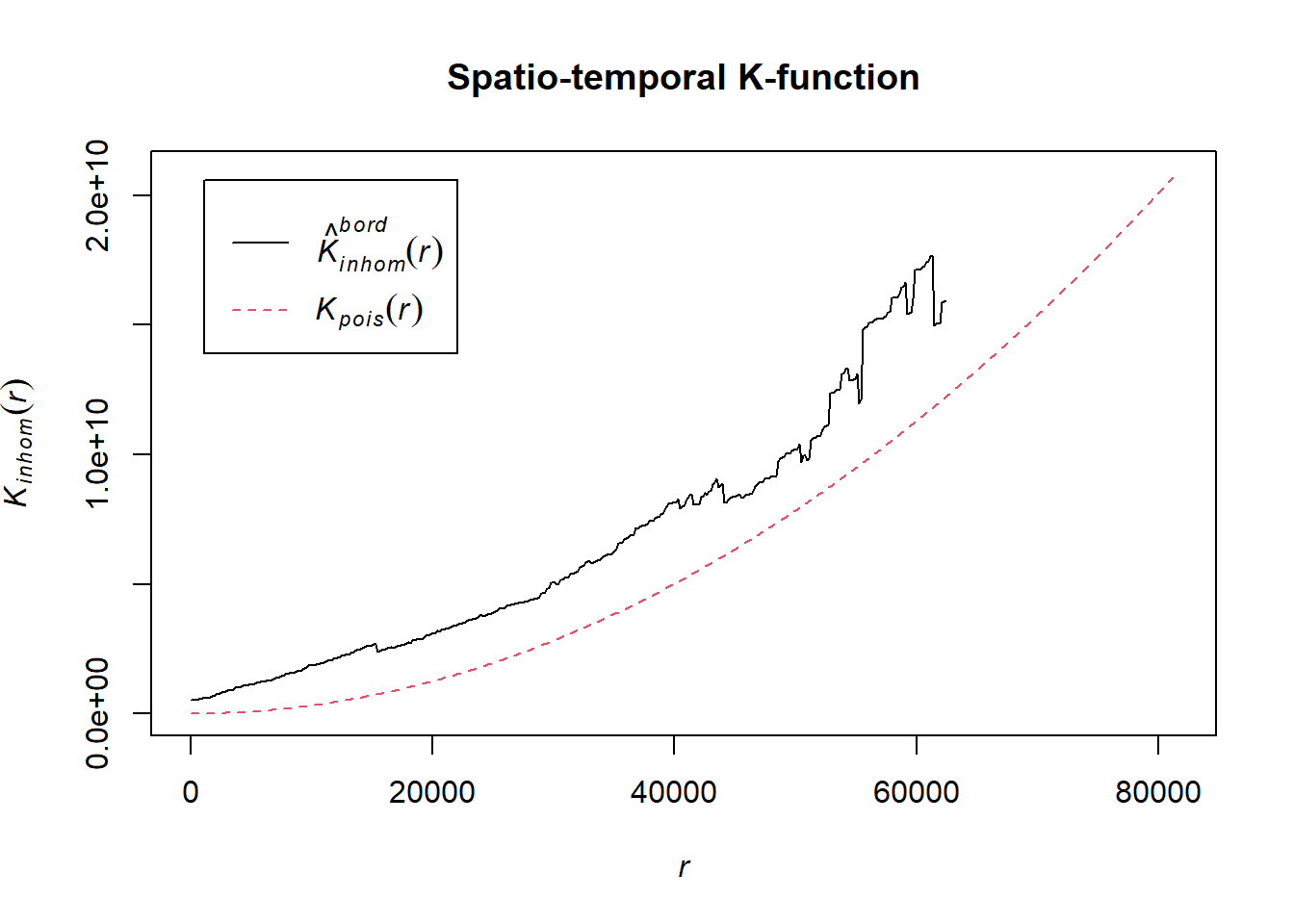
# Perform the CSR test with 99 simulations
K_ck.csr <- envelope(acled_spatio_ppp_owin, Kinhom, nsim=99, correction="border", parallel = parallel::detectCores())Generating 99 simulations of CSR ...
1, 2, 3, 4, 5, 6, 7, 8, 9, 10, 11, 12, 13, 14, 15, 16, 17, 18, 19, 20,
21, 22, 23, 24, 25, 26, 27, 28, 29, 30, 31, 32, 33, 34, 35, 36, 37, 38, 39, 40,
41, 42, 43, 44, 45, 46, 47, 48, 49, 50, 51, 52, 53, 54, 55, 56, 57, 58, 59, 60,
61, 62, 63, 64, 65, 66, 67, 68, 69, 70, 71, 72, 73, 74, 75, 76, 77, 78, 79, 80,
81, 82, 83, 84, 85, 86, 87, 88, 89, 90, 91, 92, 93, 94, 95, 96, 97, 98,
99.
Done.# Plot the envelope with the observed K-function
plot(K_ck.csr, main="Spatio-temporal K-function Envelope", legend=TRUE)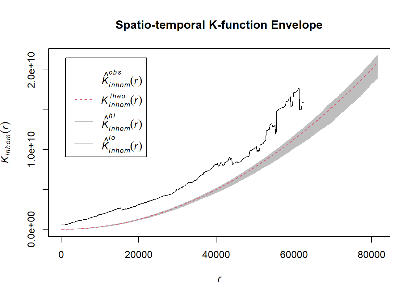
# Assuming `acled_spatio_ppp_owin` is your spatio-temporal point pattern object:
acled_spatio_ppp_owin <- sagaing_acled_quarters_2024_ppp[sagaing_owin]
K_st <- Kinhom(acled_spatio_ppp_owin, correction="border")
# Plot the result for visual inspection
plot(K_st, main = "Spatio-temporal K-function", legend=TRUE)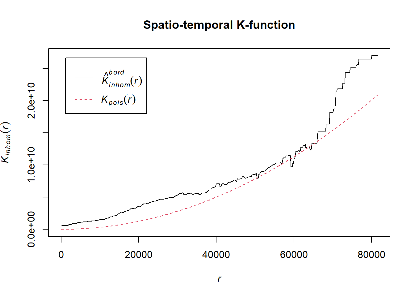
# Perform the CSR test with 99 simulations
K_ck.csr <- envelope(acled_spatio_ppp_owin, Kinhom, nsim=99, correction="border", parallel = parallel::detectCores())Generating 99 simulations of CSR ...
1, 2, 3, 4, 5, 6, 7, 8, 9, 10, 11, 12, 13, 14, 15, 16, 17, 18, 19, 20,
21, 22, 23, 24, 25, 26, 27, 28, 29, 30, 31, 32, 33, 34, 35, 36, 37, 38, 39, 40,
41, 42, 43, 44, 45, 46, 47, 48, 49, 50, 51, 52, 53, 54, 55, 56, 57, 58, 59, 60,
61, 62, 63, 64, 65, 66, 67, 68, 69, 70, 71, 72, 73, 74, 75, 76, 77, 78, 79, 80,
81, 82, 83, 84, 85, 86, 87, 88, 89, 90, 91, 92, 93, 94, 95, 96, 97, 98,
99.
Done.# Plot the envelope with the observed K-function
plot(K_ck.csr, main="Spatio-temporal K-function Envelope", legend=TRUE)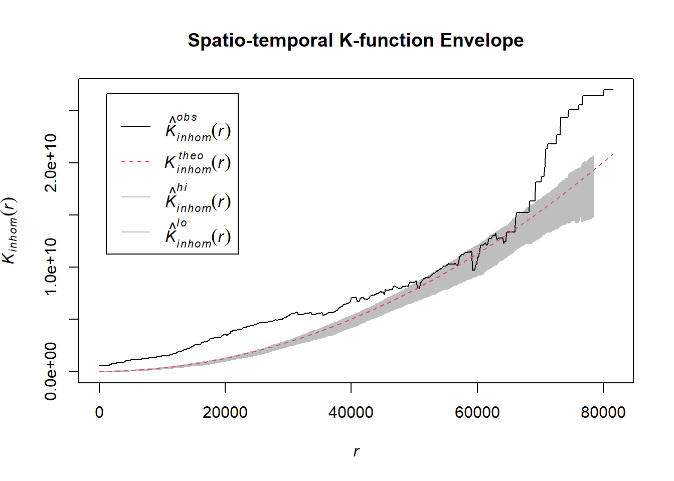
1.8.4.3.2 Strategic developments
Example <- "Strategic developments"
sagaing_acled_quarters_2021_ppp <- as.ppp(sagaing_acled_sf %>%
filter(year == 2021 & event_type == Example) %>%
select(q))
sagaing_acled_quarters_2022_ppp <- as.ppp(sagaing_acled_sf %>%
filter(year == 2022 & event_type == Example) %>%
select(q))
sagaing_acled_quarters_2023_ppp <- as.ppp(sagaing_acled_sf %>%
filter(year == 2023 & event_type == Example) %>%
select(q))
sagaing_acled_quarters_2024_ppp <- as.ppp(sagaing_acled_sf %>%
filter(year == 2024 & event_type == Example) %>%
select(q))# Assuming `acled_spatio_ppp_owin` is your spatio-temporal point pattern object:
acled_spatio_ppp_owin <- sagaing_acled_quarters_2021_ppp[sagaing_owin]
K_st <- Kinhom(acled_spatio_ppp_owin, correction="border")
# Plot the result for visual inspection
plot(K_st, main = "Spatio-temporal K-function", legend=TRUE)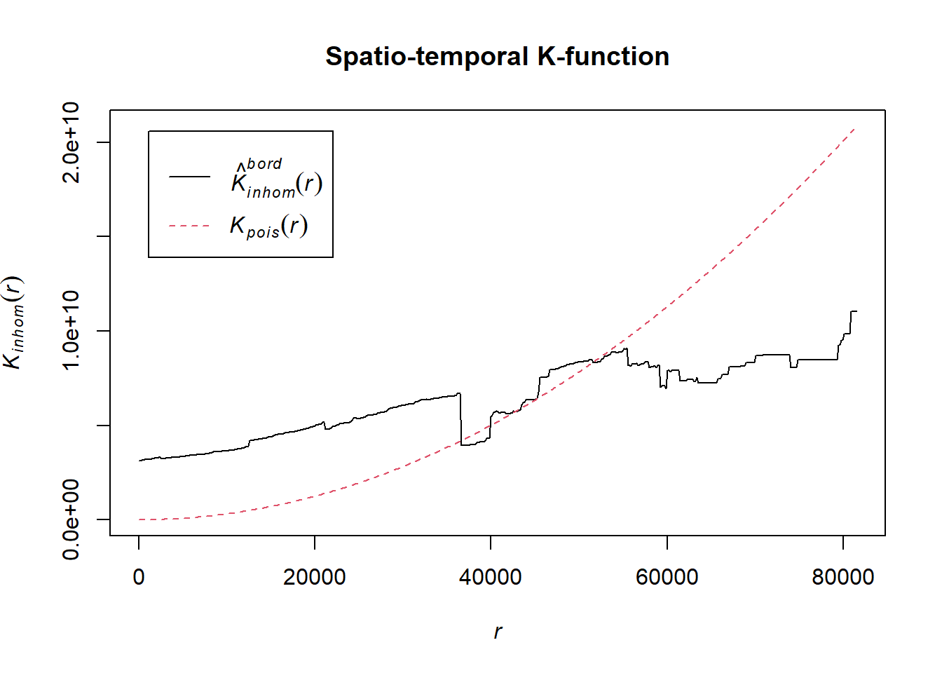
# Perform the CSR test with 99 simulations
K_ck.csr <- envelope(acled_spatio_ppp_owin, Kinhom, nsim=99, correction="border", parallel = parallel::detectCores())Generating 99 simulations of CSR ...
1, 2, 3, 4, 5, 6, 7, 8, 9, 10, 11, 12, 13, 14, 15, 16, 17, 18, 19, 20,
21, 22, 23, 24, 25, 26, 27, 28, 29, 30, 31, 32, 33, 34, 35, 36, 37, 38, 39, 40,
41, 42, 43, 44, 45, 46, 47, 48, 49, 50, 51, 52, 53, 54, 55, 56, 57, 58, 59, 60,
61, 62, 63, 64, 65, 66, 67, 68, 69, 70, 71, 72, 73, 74, 75, 76, 77, 78, 79, 80,
81, 82, 83, 84, 85, 86, 87, 88, 89, 90, 91, 92, 93, 94, 95, 96, 97, 98,
99.
Done.# Plot the envelope with the observed K-function
plot(K_ck.csr, main="Spatio-temporal K-function Envelope", legend=TRUE)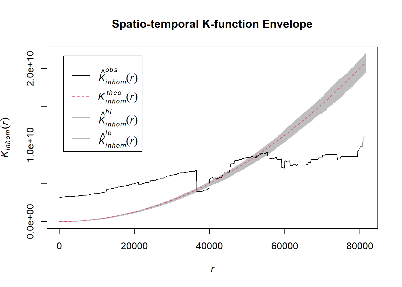
# Assuming `acled_spatio_ppp_owin` is your spatio-temporal point pattern object:
acled_spatio_ppp_owin <- sagaing_acled_quarters_2022_ppp[sagaing_owin]
K_st <- Kinhom(acled_spatio_ppp_owin, correction="border")
# Plot the result for visual inspection
plot(K_st, main = "Spatio-temporal K-function", legend=TRUE)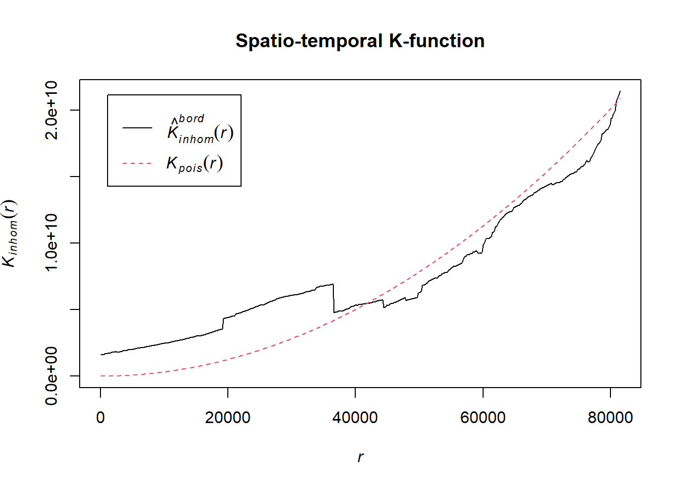
# Perform the CSR test with 99 simulations
K_ck.csr <- envelope(acled_spatio_ppp_owin, Kinhom, nsim=99, correction="border", parallel = parallel::detectCores())Generating 99 simulations of CSR ...
1, 2, 3, 4, 5, 6, 7, 8, 9, 10, 11, 12, 13, 14, 15, 16, 17, 18, 19, 20,
21, 22, 23, 24, 25, 26, 27, 28, 29, 30, 31, 32, 33, 34, 35, 36, 37, 38, 39, 40,
41, 42, 43, 44, 45, 46, 47, 48, 49, 50, 51, 52, 53, 54, 55, 56, 57, 58, 59, 60,
61, 62, 63, 64, 65, 66, 67, 68, 69, 70, 71, 72, 73, 74, 75, 76, 77, 78, 79, 80,
81, 82, 83, 84, 85, 86, 87, 88, 89, 90, 91, 92, 93, 94, 95, 96, 97, 98,
99.
Done.# Plot the envelope with the observed K-function
plot(K_ck.csr, main="Spatio-temporal K-function Envelope", legend=TRUE)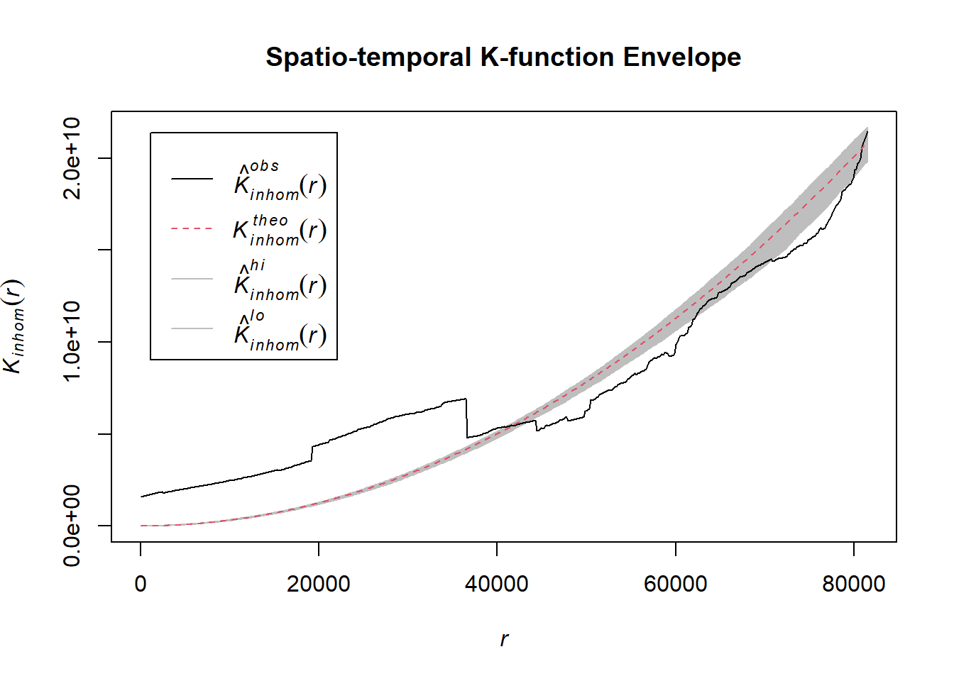
# Assuming `acled_spatio_ppp_owin` is your spatio-temporal point pattern object:
acled_spatio_ppp_owin <- sagaing_acled_quarters_2023_ppp[sagaing_owin]
K_st <- Kinhom(acled_spatio_ppp_owin, correction="border")
# Plot the result for visual inspection
plot(K_st, main = "Spatio-temporal K-function", legend=TRUE)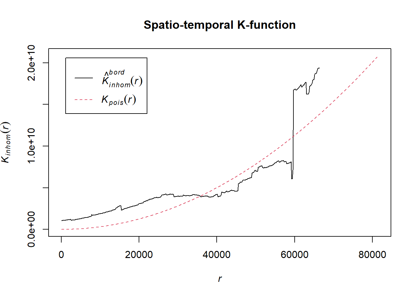
# Perform the CSR test with 99 simulations
K_ck.csr <- envelope(acled_spatio_ppp_owin, Kinhom, nsim=99, correction="border", parallel = parallel::detectCores())Generating 99 simulations of CSR ...
1, 2, 3, 4, 5, 6, 7, 8, 9, 10, 11, 12, 13, 14, 15, 16, 17, 18, 19, 20,
21, 22, 23, 24, 25, 26, 27, 28, 29, 30, 31, 32, 33, 34, 35, 36, 37, 38, 39, 40,
41, 42, 43, 44, 45, 46, 47, 48, 49, 50, 51, 52, 53, 54, 55, 56, 57, 58, 59, 60,
61, 62, 63, 64, 65, 66, 67, 68, 69, 70, 71, 72, 73, 74, 75, 76, 77, 78, 79, 80,
81, 82, 83, 84, 85, 86, 87, 88, 89, 90, 91, 92, 93, 94, 95, 96, 97, 98,
99.
Done.# Plot the envelope with the observed K-function
plot(K_ck.csr, main="Spatio-temporal K-function Envelope", legend=TRUE)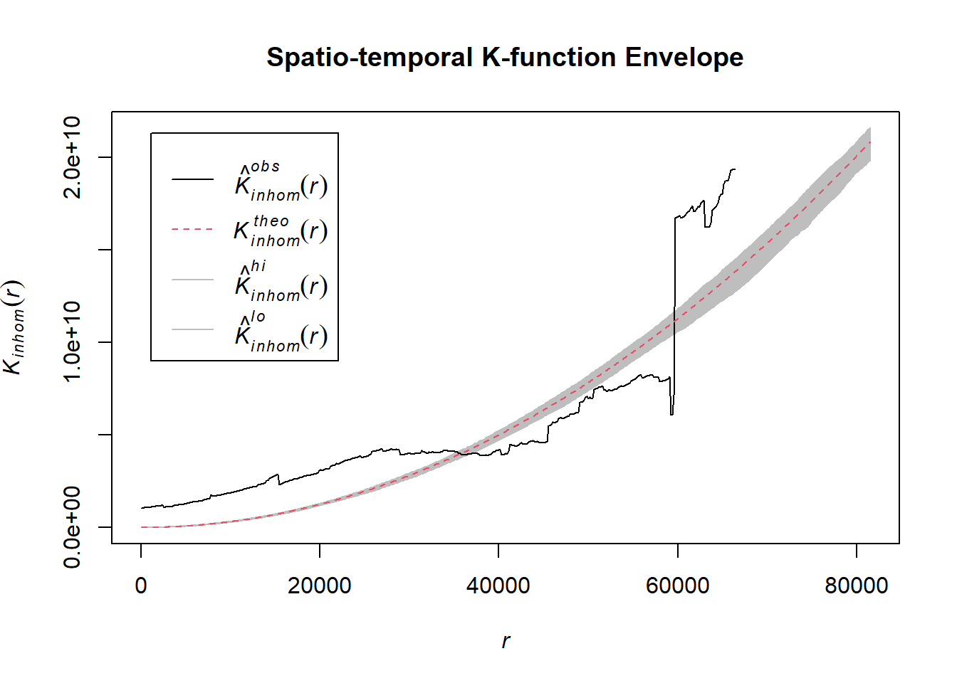
# Assuming `acled_spatio_ppp_owin` is your spatio-temporal point pattern object:
acled_spatio_ppp_owin <- sagaing_acled_quarters_2024_ppp[sagaing_owin]
K_st <- Kinhom(acled_spatio_ppp_owin, correction="border")
# Plot the result for visual inspection
plot(K_st, main = "Spatio-temporal K-function", legend=TRUE)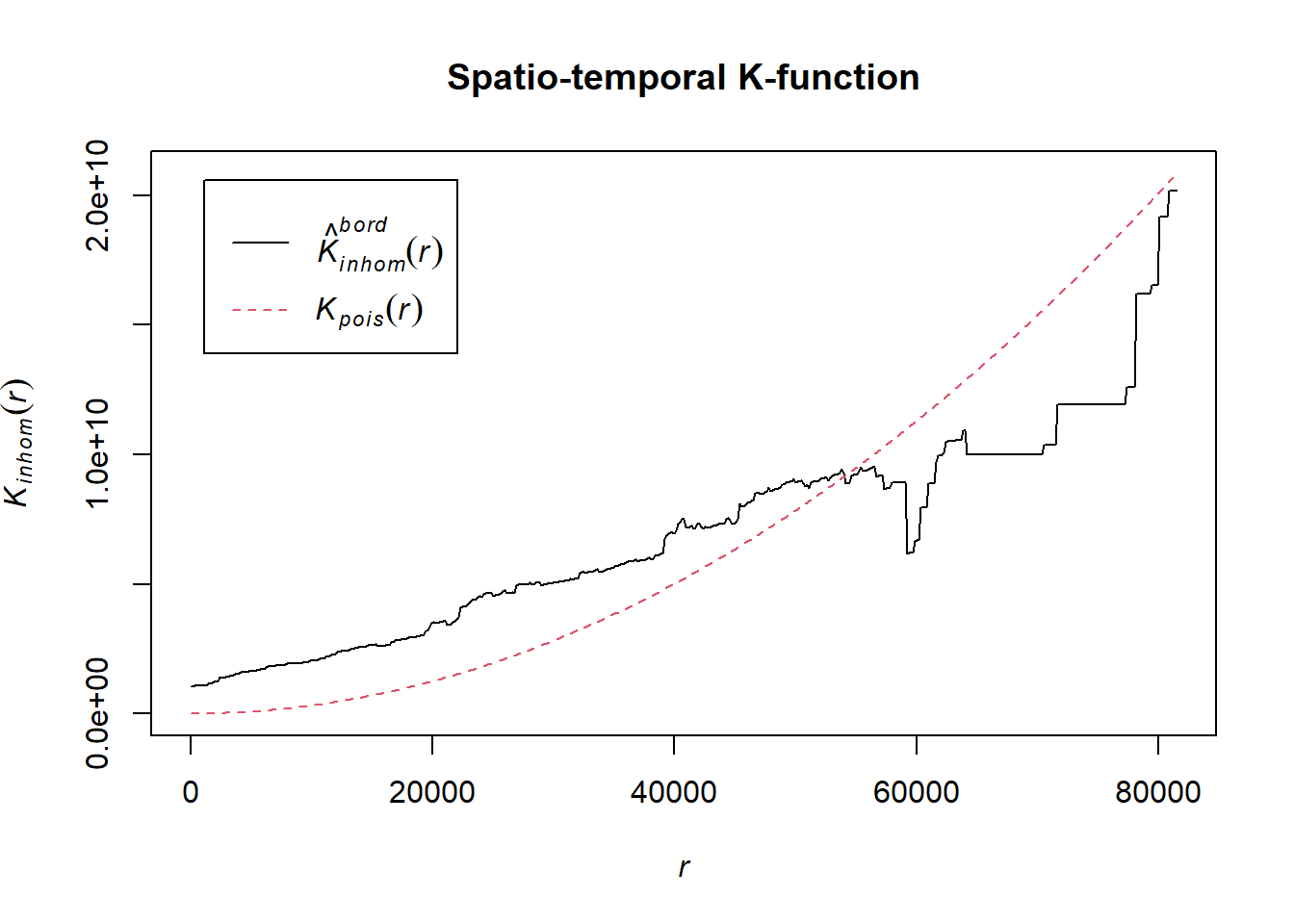
# Perform the CSR test with 99 simulations
K_ck.csr <- envelope(acled_spatio_ppp_owin, Kinhom, nsim=99, correction="border", parallel = parallel::detectCores())Generating 99 simulations of CSR ...
1, 2, 3, 4, 5, 6, 7, 8, 9, 10, 11, 12, 13, 14, 15, 16, 17, 18, 19, 20,
21, 22, 23, 24, 25, 26, 27, 28, 29, 30, 31, 32, 33, 34, 35, 36, 37, 38, 39, 40,
41, 42, 43, 44, 45, 46, 47, 48, 49, 50, 51, 52, 53, 54, 55, 56, 57, 58, 59, 60,
61, 62, 63, 64, 65, 66, 67, 68, 69, 70, 71, 72, 73, 74, 75, 76, 77, 78, 79, 80,
81, 82, 83, 84, 85, 86, 87, 88, 89, 90, 91, 92, 93, 94, 95, 96, 97, 98,
99.
Done.# Plot the envelope with the observed K-function
plot(K_ck.csr, main="Spatio-temporal K-function Envelope", legend=TRUE)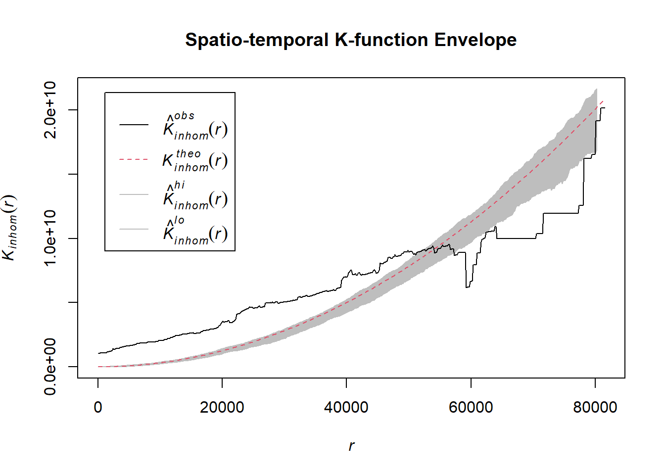
1.8.4.3.3 Battles
Example <- "Battles"
sagaing_acled_quarters_2021_ppp <- as.ppp(sagaing_acled_sf %>%
filter(year == 2021 & event_type == Example) %>%
select(q))
sagaing_acled_quarters_2022_ppp <- as.ppp(sagaing_acled_sf %>%
filter(year == 2022 & event_type == Example) %>%
select(q))
sagaing_acled_quarters_2023_ppp <- as.ppp(sagaing_acled_sf %>%
filter(year == 2023 & event_type == Example) %>%
select(q))
sagaing_acled_quarters_2024_ppp <- as.ppp(sagaing_acled_sf %>%
filter(year == 2024 & event_type == Example) %>%
select(q))# Assuming `acled_spatio_ppp_owin` is your spatio-temporal point pattern object:
acled_spatio_ppp_owin <- sagaing_acled_quarters_2021_ppp[sagaing_owin]
K_st <- Kinhom(acled_spatio_ppp_owin, correction="border")
# Plot the result for visual inspection
plot(K_st, main = "Spatio-temporal K-function", legend=TRUE)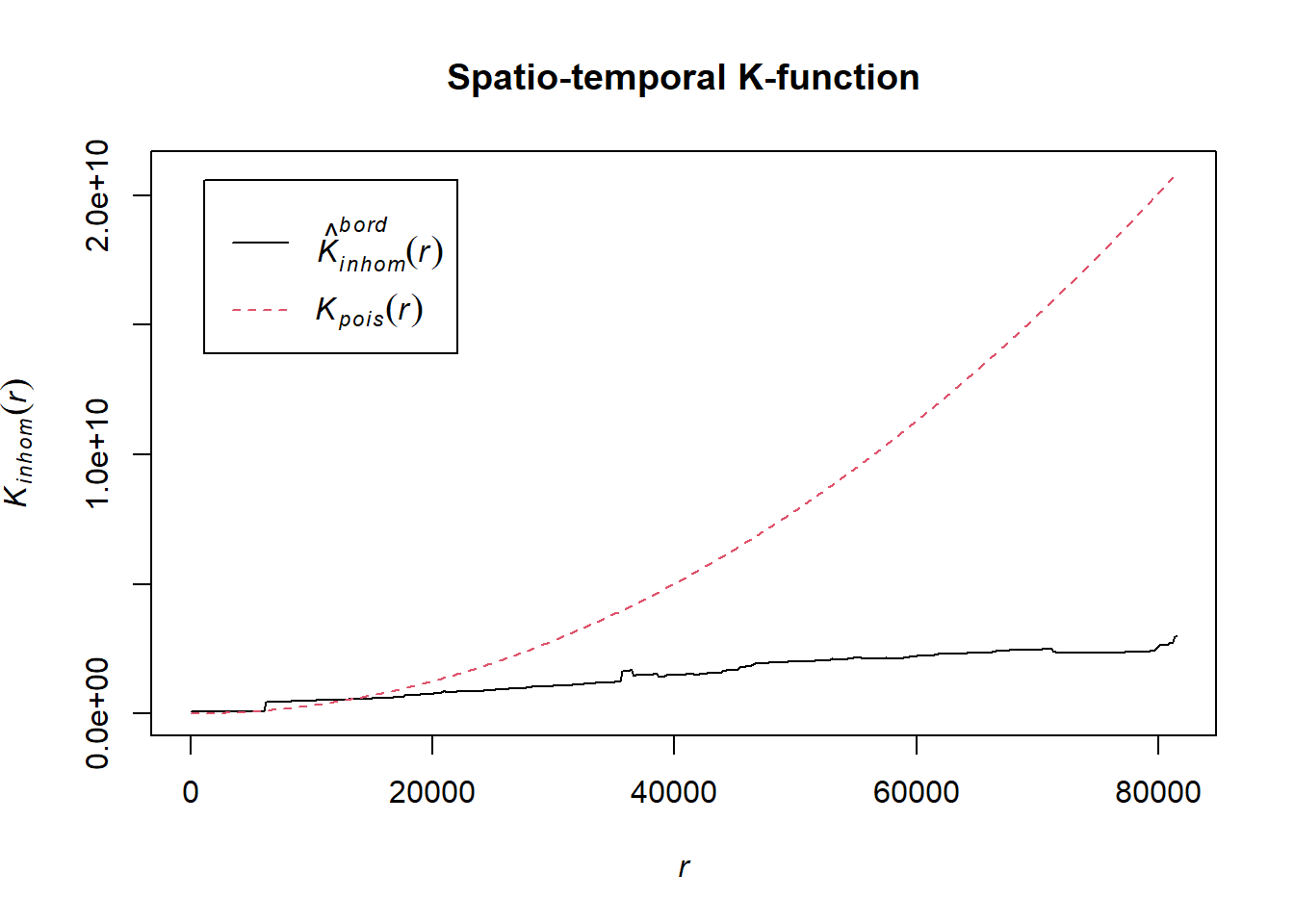
# Perform the CSR test with 99 simulations
K_ck.csr <- envelope(acled_spatio_ppp_owin, Kinhom, nsim=99, correction="border", parallel = parallel::detectCores())Generating 99 simulations of CSR ...
1, 2, 3, 4, 5, 6, 7, 8, 9, 10, 11, 12, 13, 14, 15, 16, 17, 18, 19, 20,
21, 22, 23, 24, 25, 26, 27, 28, 29, 30, 31, 32, 33, 34, 35, 36, 37, 38, 39, 40,
41, 42, 43, 44, 45, 46, 47, 48, 49, 50, 51, 52, 53, 54, 55, 56, 57, 58, 59, 60,
61, 62, 63, 64, 65, 66, 67, 68, 69, 70, 71, 72, 73, 74, 75, 76, 77, 78, 79, 80,
81, 82, 83, 84, 85, 86, 87, 88, 89, 90, 91, 92, 93, 94, 95, 96, 97, 98,
99.
Done.# Plot the envelope with the observed K-function
plot(K_ck.csr, main="Spatio-temporal K-function Envelope", legend=TRUE)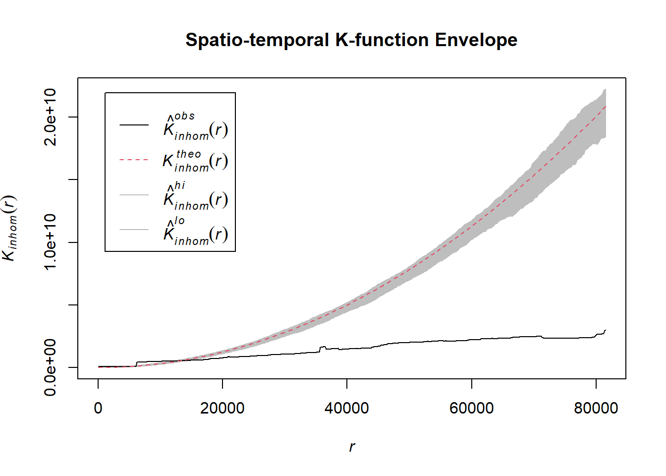
# Assuming `acled_spatio_ppp_owin` is your spatio-temporal point pattern object:
acled_spatio_ppp_owin <- sagaing_acled_quarters_2022_ppp[sagaing_owin]
K_st <- Kinhom(acled_spatio_ppp_owin, correction="border")
# Plot the result for visual inspection
plot(K_st, main = "Spatio-temporal K-function", legend=TRUE)
# Perform the CSR test with 99 simulations
K_ck.csr <- envelope(acled_spatio_ppp_owin, Kinhom, nsim=99, correction="border", parallel = parallel::detectCores())Generating 99 simulations of CSR ...
1, 2, 3, 4, 5, 6, 7, 8, 9, 10, 11, 12, 13, 14, 15, 16, 17, 18, 19, 20,
21, 22, 23, 24, 25, 26, 27, 28, 29, 30, 31, 32, 33, 34, 35, 36, 37, 38, 39, 40,
41, 42, 43, 44, 45, 46, 47, 48, 49, 50, 51, 52, 53, 54, 55, 56, 57, 58, 59, 60,
61, 62, 63, 64, 65, 66, 67, 68, 69, 70, 71, 72, 73, 74, 75, 76, 77, 78, 79, 80,
81, 82, 83, 84, 85, 86, 87, 88, 89, 90, 91, 92, 93, 94, 95, 96, 97, 98,
99.
Done.# Plot the envelope with the observed K-function
plot(K_ck.csr, main="Spatio-temporal K-function Envelope", legend=TRUE)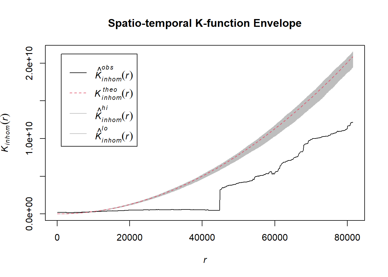
# Assuming `acled_spatio_ppp_owin` is your spatio-temporal point pattern object:
acled_spatio_ppp_owin <- sagaing_acled_quarters_2023_ppp[sagaing_owin]
K_st <- Kinhom(acled_spatio_ppp_owin, correction="border")
# Plot the result for visual inspection
plot(K_st, main = "Spatio-temporal K-function", legend=TRUE)
# Perform the CSR test with 99 simulations
K_ck.csr <- envelope(acled_spatio_ppp_owin, Kinhom, nsim=99, correction="border", parallel = parallel::detectCores())Generating 99 simulations of CSR ...
1, 2, 3, 4, 5, 6, 7, 8, 9, 10, 11, 12, 13, 14, 15, 16, 17, 18, 19, 20,
21, 22, 23, 24, 25, 26, 27, 28, 29, 30, 31, 32, 33, 34, 35, 36, 37, 38, 39, 40,
41, 42, 43, 44, 45, 46, 47, 48, 49, 50, 51, 52, 53, 54, 55, 56, 57, 58, 59, 60,
61, 62, 63, 64, 65, 66, 67, 68, 69, 70, 71, 72, 73, 74, 75, 76, 77, 78, 79, 80,
81, 82, 83, 84, 85, 86, 87, 88, 89, 90, 91, 92, 93, 94, 95, 96, 97, 98,
99.
Done.# Plot the envelope with the observed K-function
plot(K_ck.csr, main="Spatio-temporal K-function Envelope", legend=TRUE)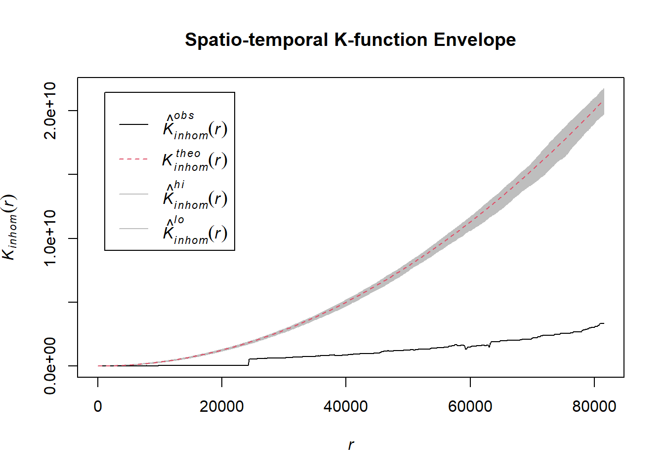
# Assuming `acled_spatio_ppp_owin` is your spatio-temporal point pattern object:
acled_spatio_ppp_owin <- sagaing_acled_quarters_2024_ppp[sagaing_owin]
K_st <- Kinhom(acled_spatio_ppp_owin, correction="border")
# Plot the result for visual inspection
plot(K_st, main = "Spatio-temporal K-function", legend=TRUE)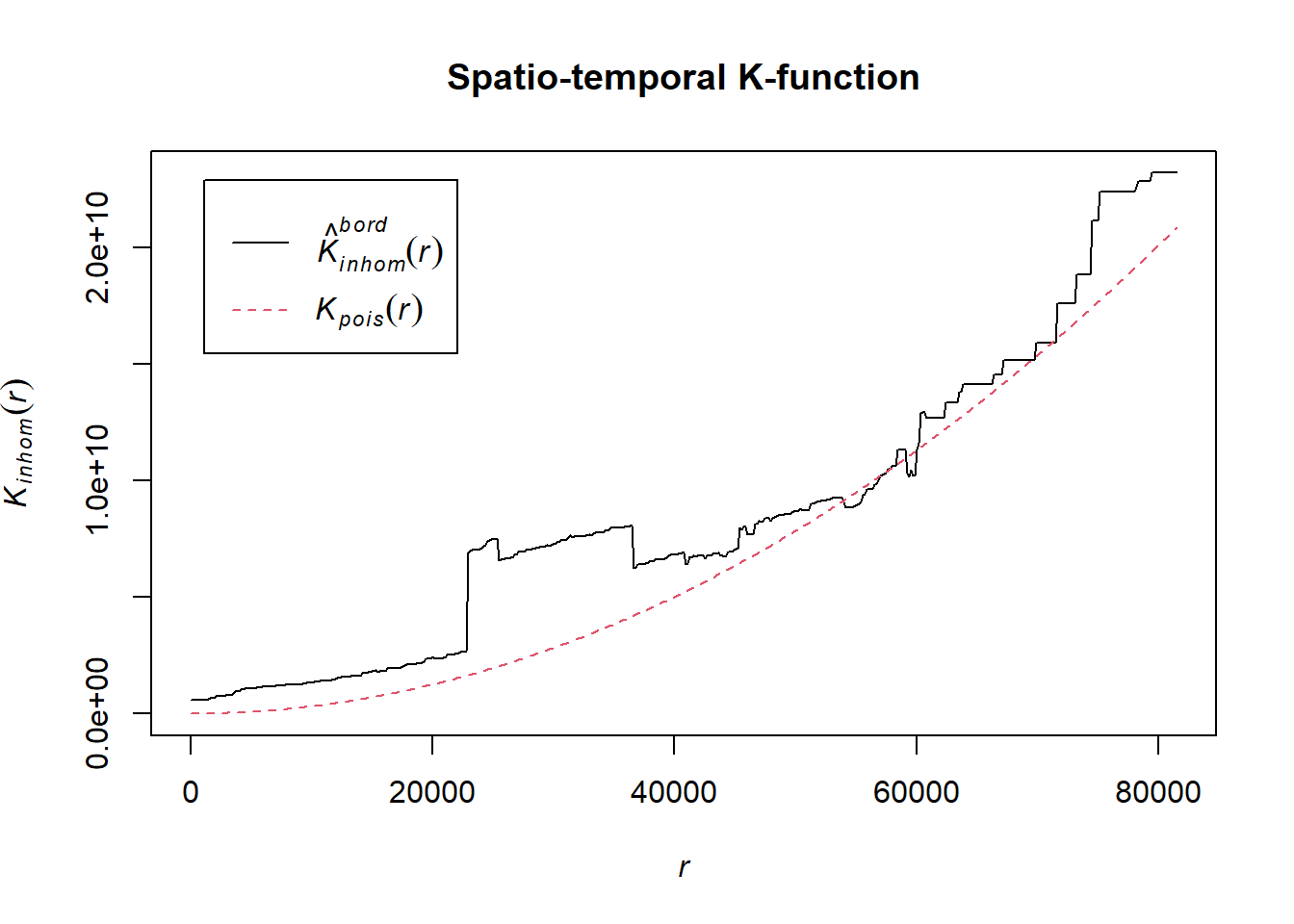
# Perform the CSR test with 99 simulations
K_ck.csr <- envelope(acled_spatio_ppp_owin, Kinhom, nsim=99, correction="border", parallel = parallel::detectCores())Generating 99 simulations of CSR ...
1, 2, 3, 4, 5, 6, 7, 8, 9, 10, 11, 12, 13, 14, 15, 16, 17, 18, 19, 20,
21, 22, 23, 24, 25, 26, 27, 28, 29, 30, 31, 32, 33, 34, 35, 36, 37, 38, 39, 40,
41, 42, 43, 44, 45, 46, 47, 48, 49, 50, 51, 52, 53, 54, 55, 56, 57, 58, 59, 60,
61, 62, 63, 64, 65, 66, 67, 68, 69, 70, 71, 72, 73, 74, 75, 76, 77, 78, 79, 80,
81, 82, 83, 84, 85, 86, 87, 88, 89, 90, 91, 92, 93, 94, 95, 96, 97, 98,
99.
Done.# Plot the envelope with the observed K-function
plot(K_ck.csr, main="Spatio-temporal K-function Envelope", legend=TRUE)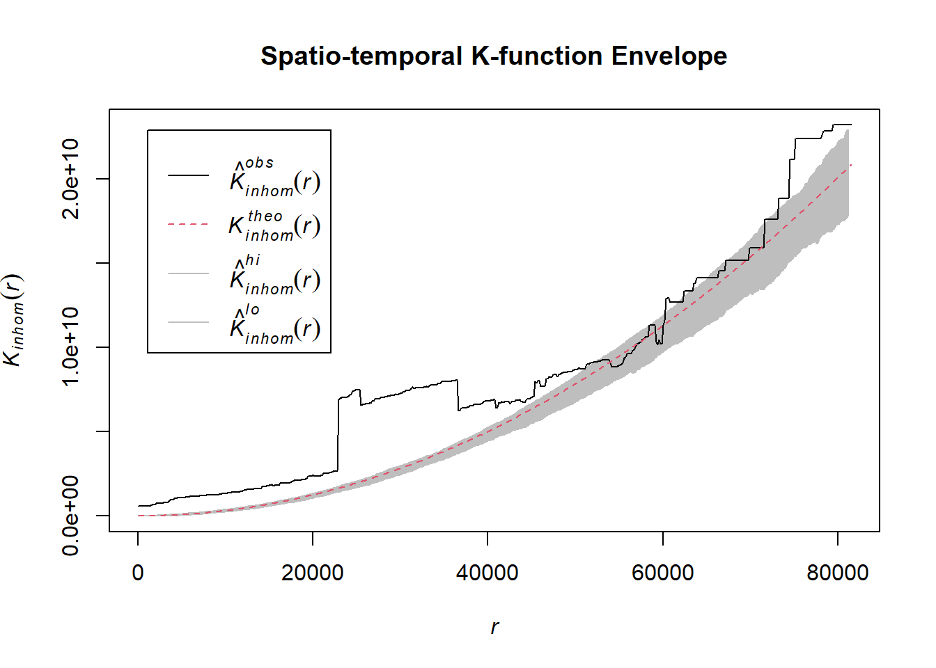
1.8.4.3.4 Violence against civilians
Example <- "Violence against civilians"
acled_quarters_2021_ppp <- as.ppp(temporal_acled_sf %>%
filter(year == 2021 & event_type == Example) %>%
select(q))
acled_quarters_2022_ppp <- as.ppp(temporal_acled_sf %>%
filter(year == 2022 & event_type == Example) %>%
select(q))
acled_quarters_2023_ppp <- as.ppp(temporal_acled_sf %>%
filter(year == 2023 & event_type == Example) %>%
select(q))
acled_quarters_2024_ppp <- as.ppp(temporal_acled_sf %>%
filter(year == 2024 & event_type == Example) %>%
select(q))# Assuming `acled_spatio_ppp_owin` is your spatio-temporal point pattern object:
acled_spatio_ppp_owin <- sagaing_acled_quarters_2021_ppp[sagaing_owin]
K_st <- Kinhom(acled_spatio_ppp_owin, correction="border")
# Plot the result for visual inspection
plot(K_st, main = "Spatio-temporal K-function", legend=TRUE)
# Perform the CSR test with 99 simulations
K_ck.csr <- envelope(acled_spatio_ppp_owin, Kinhom, nsim=99, correction="border", parallel = parallel::detectCores())Generating 99 simulations of CSR ...
1, 2, 3, 4, 5, 6, 7, 8, 9, 10, 11, 12, 13, 14, 15, 16, 17, 18, 19, 20,
21, 22, 23, 24, 25, 26, 27, 28, 29, 30, 31, 32, 33, 34, 35, 36, 37, 38, 39, 40,
41, 42, 43, 44, 45, 46, 47, 48, 49, 50, 51, 52, 53, 54, 55, 56, 57, 58, 59, 60,
61, 62, 63, 64, 65, 66, 67, 68, 69, 70, 71, 72, 73, 74, 75, 76, 77, 78, 79, 80,
81, 82, 83, 84, 85, 86, 87, 88, 89, 90, 91, 92, 93, 94, 95, 96, 97, 98,
99.
Done.# Plot the envelope with the observed K-function
plot(K_ck.csr, main="Spatio-temporal K-function Envelope", legend=TRUE)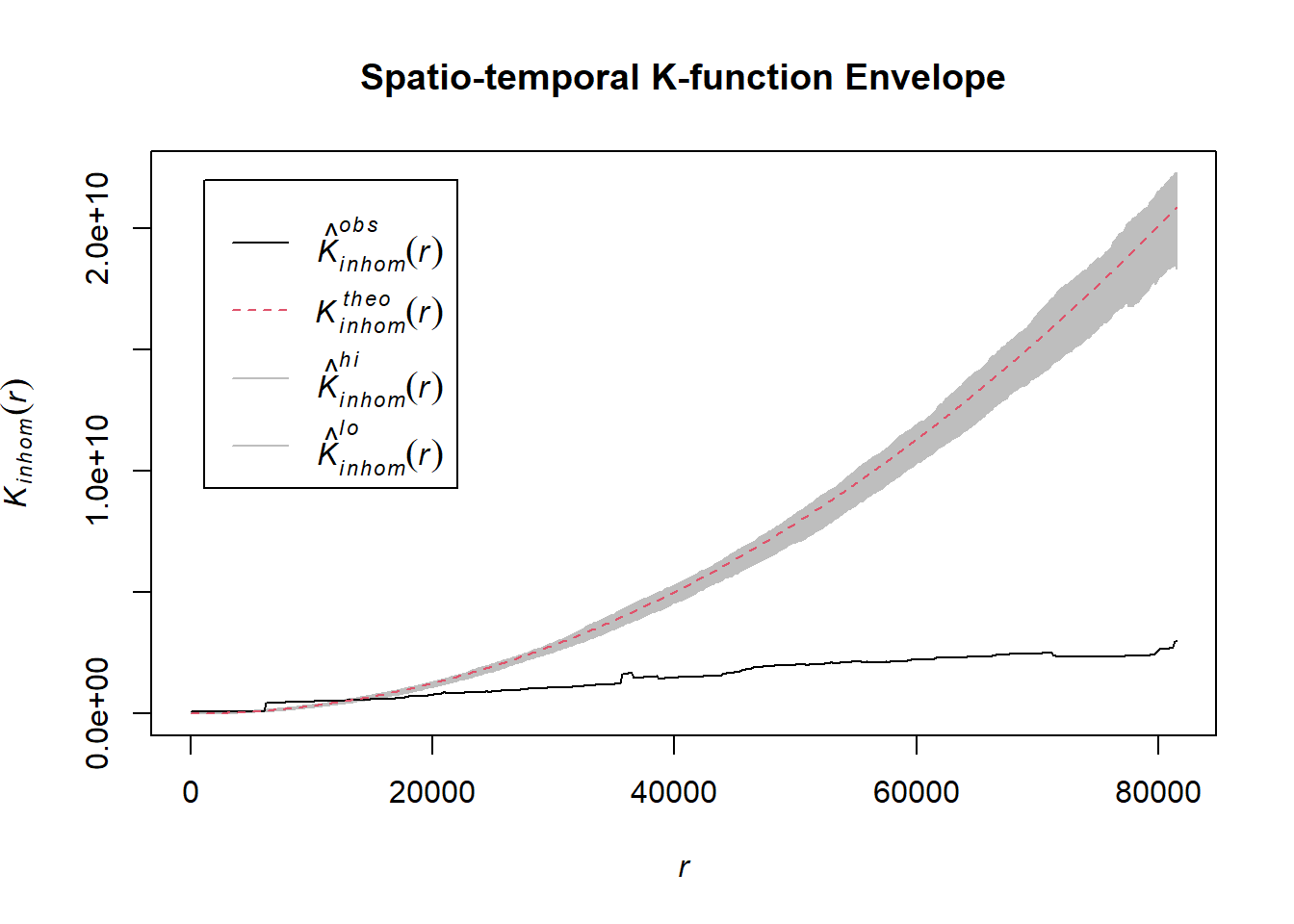
# Assuming `acled_spatio_ppp_owin` is your spatio-temporal point pattern object:
acled_spatio_ppp_owin <- sagaing_acled_quarters_2022_ppp[sagaing_owin]
K_st <- Kinhom(acled_spatio_ppp_owin, correction="border")
# Plot the result for visual inspection
plot(K_st, main = "Spatio-temporal K-function", legend=TRUE)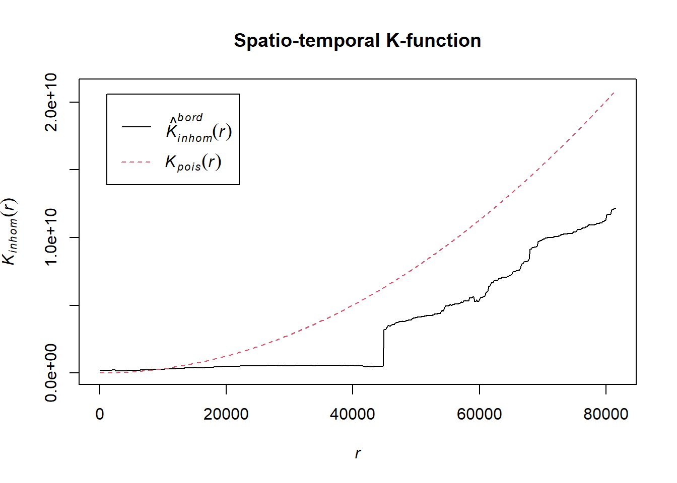
# Perform the CSR test with 99 simulations
K_ck.csr <- envelope(acled_spatio_ppp_owin, Kinhom, nsim=99, correction="border", parallel = parallel::detectCores())Generating 99 simulations of CSR ...
1, 2, 3, 4, 5, 6, 7, 8, 9, 10, 11, 12, 13, 14, 15, 16, 17, 18, 19, 20,
21, 22, 23, 24, 25, 26, 27, 28, 29, 30, 31, 32, 33, 34, 35, 36, 37, 38, 39, 40,
41, 42, 43, 44, 45, 46, 47, 48, 49, 50, 51, 52, 53, 54, 55, 56, 57, 58, 59, 60,
61, 62, 63, 64, 65, 66, 67, 68, 69, 70, 71, 72, 73, 74, 75, 76, 77, 78, 79, 80,
81, 82, 83, 84, 85, 86, 87, 88, 89, 90, 91, 92, 93, 94, 95, 96, 97, 98,
99.
Done.# Plot the envelope with the observed K-function
plot(K_ck.csr, main="Spatio-temporal K-function Envelope", legend=TRUE)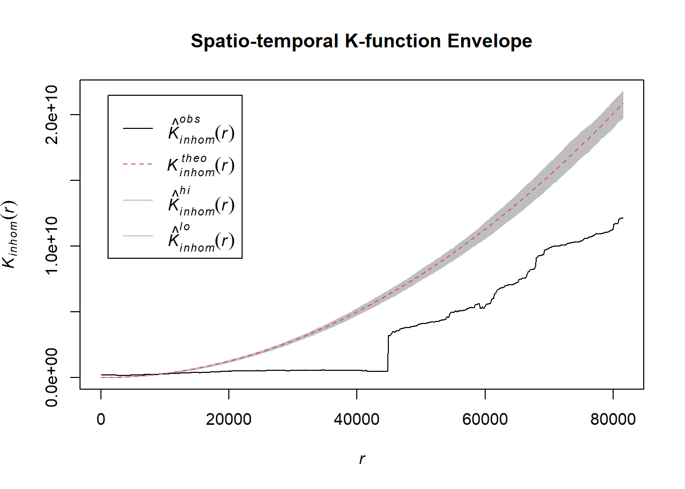
# Assuming `acled_spatio_ppp_owin` is your spatio-temporal point pattern object:
acled_spatio_ppp_owin <- sagaing_acled_quarters_2023_ppp[sagaing_owin]
K_st <- Kinhom(acled_spatio_ppp_owin, correction="border")
# Plot the result for visual inspection
plot(K_st, main = "Spatio-temporal K-function", legend=TRUE)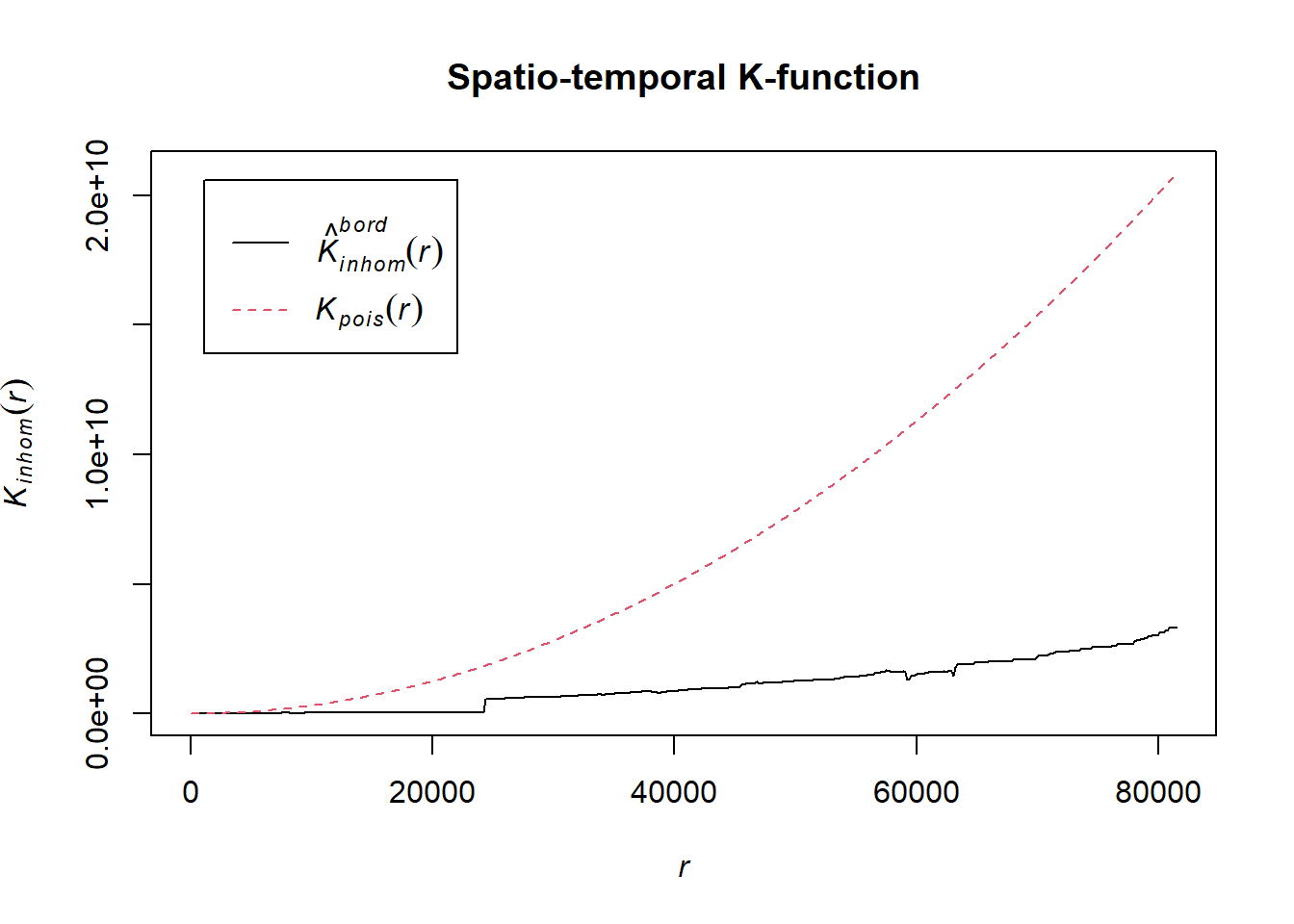
# Perform the CSR test with 99 simulations
K_ck.csr <- envelope(acled_spatio_ppp_owin, Kinhom, nsim=99, correction="border", parallel = parallel::detectCores())Generating 99 simulations of CSR ...
1, 2, 3, 4, 5, 6, 7, 8, 9, 10, 11, 12, 13, 14, 15, 16, 17, 18, 19, 20,
21, 22, 23, 24, 25, 26, 27, 28, 29, 30, 31, 32, 33, 34, 35, 36, 37, 38, 39, 40,
41, 42, 43, 44, 45, 46, 47, 48, 49, 50, 51, 52, 53, 54, 55, 56, 57, 58, 59, 60,
61, 62, 63, 64, 65, 66, 67, 68, 69, 70, 71, 72, 73, 74, 75, 76, 77, 78, 79, 80,
81, 82, 83, 84, 85, 86, 87, 88, 89, 90, 91, 92, 93, 94, 95, 96, 97, 98,
99.
Done.# Plot the envelope with the observed K-function
plot(K_ck.csr, main="Spatio-temporal K-function Envelope", legend=TRUE)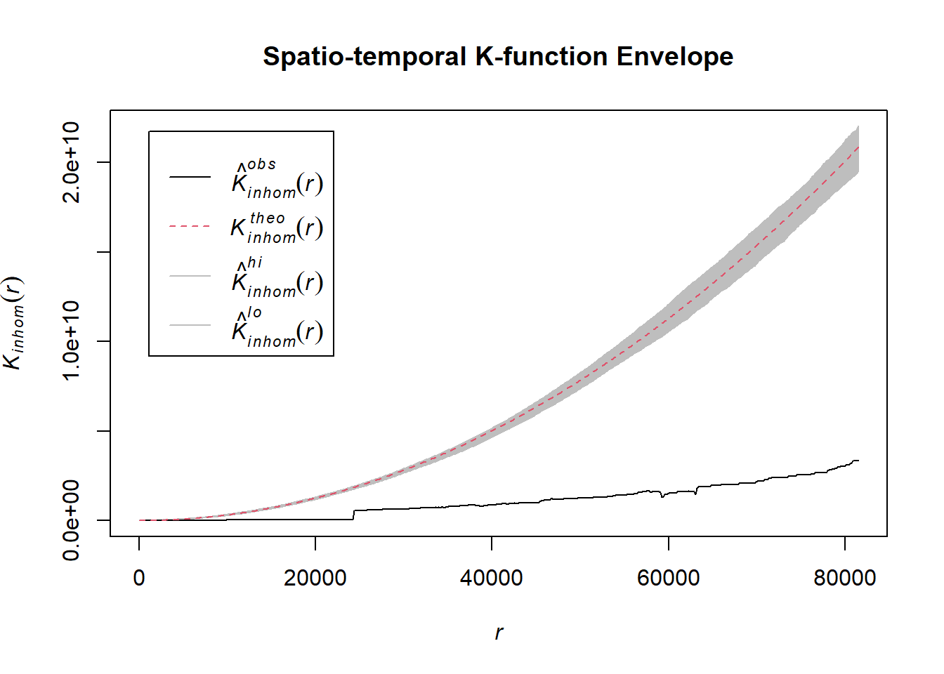
# Assuming `acled_spatio_ppp_owin` is your spatio-temporal point pattern object:
acled_spatio_ppp_owin <- sagaing_acled_quarters_2024_ppp[sagaing_owin]
K_st <- Kinhom(acled_spatio_ppp_owin, correction="border")
# Plot the result for visual inspection
plot(K_st, main = "Spatio-temporal K-function", legend=TRUE)
# Perform the CSR test with 99 simulations
K_ck.csr <- envelope(acled_spatio_ppp_owin, Kinhom, nsim=99, correction="border", parallel = parallel::detectCores())Generating 99 simulations of CSR ...
1, 2, 3, 4, 5, 6, 7, 8, 9, 10, 11, 12, 13, 14, 15, 16, 17, 18, 19, 20,
21, 22, 23, 24, 25, 26, 27, 28, 29, 30, 31, 32, 33, 34, 35, 36, 37, 38, 39, 40,
41, 42, 43, 44, 45, 46, 47, 48, 49, 50, 51, 52, 53, 54, 55, 56, 57, 58, 59, 60,
61, 62, 63, 64, 65, 66, 67, 68, 69, 70, 71, 72, 73, 74, 75, 76, 77, 78, 79, 80,
81, 82, 83, 84, 85, 86, 87, 88, 89, 90, 91, 92, 93, 94, 95, 96, 97, 98,
99.
Done.# Plot the envelope with the observed K-function
plot(K_ck.csr, main="Spatio-temporal K-function Envelope", legend=TRUE)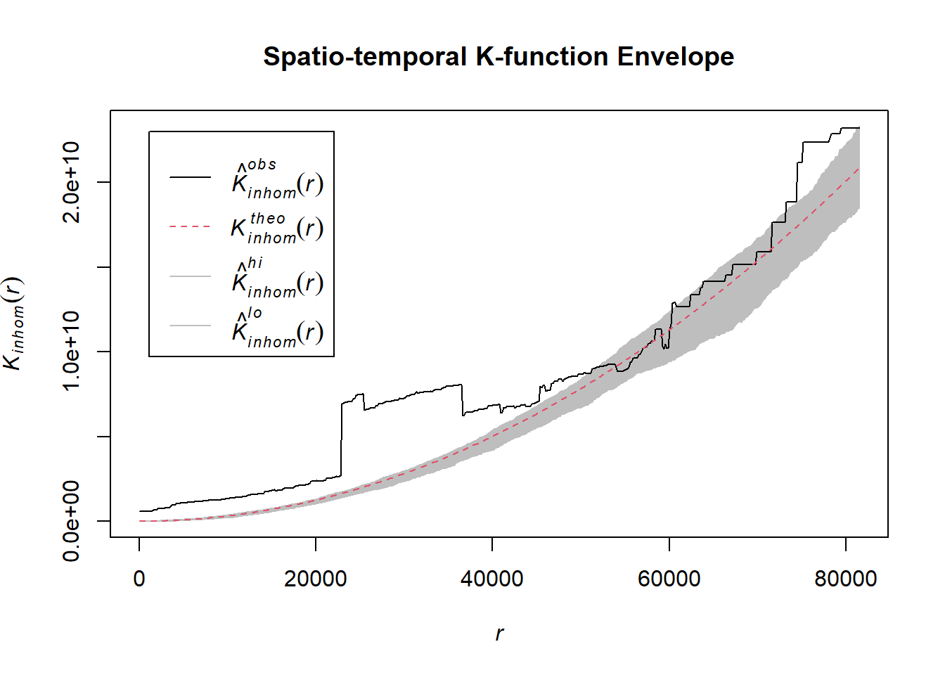
1.8.4.4 Mandalay Region
mandalay_acled_sf <- temporal_acled_sf %>% filter(admin1 == "Mandalay")
tm_shape(mandalay_sf)+
tm_polygons() +
tm_shape(mandalay_acled_sf) +
tm_dots(size=0.1) +
tm_facets(by="quarter",
free.coords=FALSE,
drop.units = TRUE) +
tm_layout(main.title = "Region and Boundaries of Mandalay",
main.title.position = "center",
main.title.size = 1,
legend.outside = TRUE,
frame = TRUE)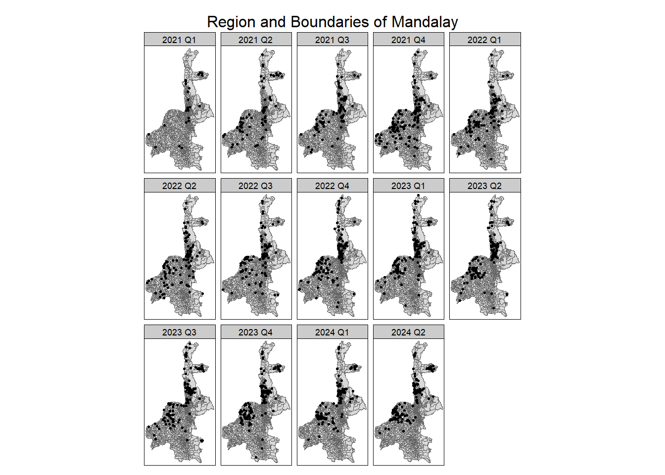
write_rds(mandalay_acled_sf, "data/rds/mandalay_acled_sf.rds")1.8.4.4.1 Explosions/Remote violence
Example <- "Explosions/Remote violence"
mandalay_acled_quarters_2021_ppp <- as.ppp(mandalay_acled_sf %>%
filter(year == 2021 & event_type == Example) %>%
select(q))
mandalay_acled_quarters_2022_ppp <- as.ppp(mandalay_acled_sf %>%
filter(year == 2022 & event_type == Example) %>%
select(q))
mandalay_acled_quarters_2023_ppp <- as.ppp(mandalay_acled_sf %>%
filter(year == 2023 & event_type == Example) %>%
select(q))
mandalay_acled_quarters_2024_ppp <- as.ppp(mandalay_acled_sf %>%
filter(year == 2024 & event_type == Example) %>%
select(q))# Assuming `acled_spatio_ppp_owin` is your spatio-temporal point pattern object:
acled_spatio_ppp_owin <- mandalay_acled_quarters_2021_ppp[mandalay_owin]
K_st <- Kinhom(acled_spatio_ppp_owin, correction="border")
# Plot the result for visual inspection
plot(K_st, main = "Spatio-temporal K-function", legend=TRUE)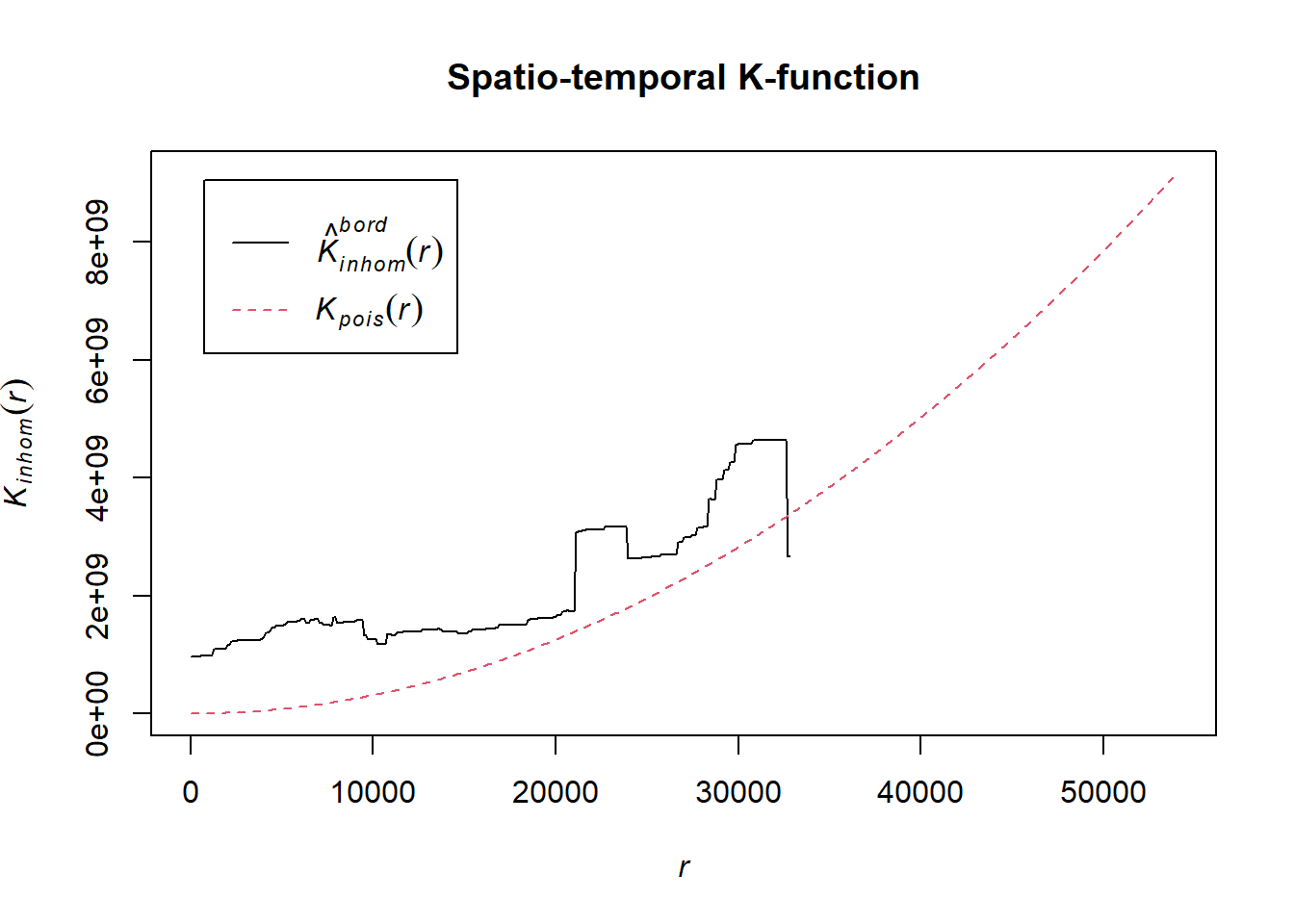
# Perform the CSR test with 99 simulations
K_ck.csr <- envelope(acled_spatio_ppp_owin, Kinhom, nsim=99, correction="border", parallel = parallel::detectCores())Generating 99 simulations of CSR ...
1, 2, 3, 4, 5, 6, 7, 8, 9, 10, 11, 12, 13, 14, 15, 16, 17, 18, 19, 20,
21, 22, 23, 24, 25, 26, 27, 28, 29, 30, 31, 32, 33, 34, 35, 36, 37, 38, 39, 40,
41, 42, 43, 44, 45, 46, 47, 48, 49, 50, 51, 52, 53, 54, 55, 56, 57, 58, 59, 60,
61, 62, 63, 64, 65, 66, 67, 68, 69, 70, 71, 72, 73, 74, 75, 76, 77, 78, 79, 80,
81, 82, 83, 84, 85, 86, 87, 88, 89, 90, 91, 92, 93, 94, 95, 96, 97, 98,
99.
Done.# Plot the envelope with the observed K-function
plot(K_ck.csr, main="Spatio-temporal K-function Envelope", legend=TRUE)
# Assuming `acled_spatio_ppp_owin` is your spatio-temporal point pattern object:
acled_spatio_ppp_owin <- mandalay_acled_quarters_2022_ppp[mandalay_owin]
K_st <- Kinhom(acled_spatio_ppp_owin, correction="border")
# Plot the result for visual inspection
plot(K_st, main = "Spatio-temporal K-function", legend=TRUE)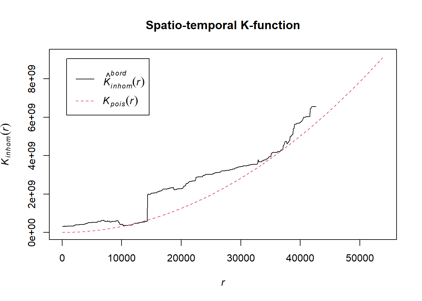
# Perform the CSR test with 99 simulations
K_ck.csr <- envelope(acled_spatio_ppp_owin, Kinhom, nsim=99, correction="border", parallel = parallel::detectCores())Generating 99 simulations of CSR ...
1, 2, 3, 4, 5, 6, 7, 8, 9, 10, 11, 12, 13, 14, 15, 16, 17, 18, 19, 20,
21, 22, 23, 24, 25, 26, 27, 28, 29, 30, 31, 32, 33, 34, 35, 36, 37, 38, 39, 40,
41, 42, 43, 44, 45, 46, 47, 48, 49, 50, 51, 52, 53, 54, 55, 56, 57, 58, 59, 60,
61, 62, 63, 64, 65, 66, 67, 68, 69, 70, 71, 72, 73, 74, 75, 76, 77, 78, 79, 80,
81, 82, 83, 84, 85, 86, 87, 88, 89, 90, 91, 92, 93, 94, 95, 96, 97, 98,
99.
Done.# Plot the envelope with the observed K-function
plot(K_ck.csr, main="Spatio-temporal K-function Envelope", legend=TRUE)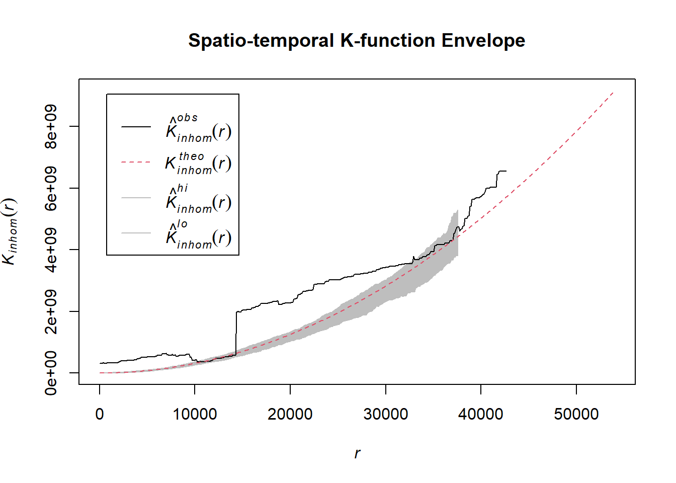
# Assuming `acled_spatio_ppp_owin` is your spatio-temporal point pattern object:
acled_spatio_ppp_owin <- mandalay_acled_quarters_2023_ppp[mandalay_owin]
K_st <- Kinhom(acled_spatio_ppp_owin, correction="border")
# Plot the result for visual inspection
plot(K_st, main = "Spatio-temporal K-function", legend=TRUE)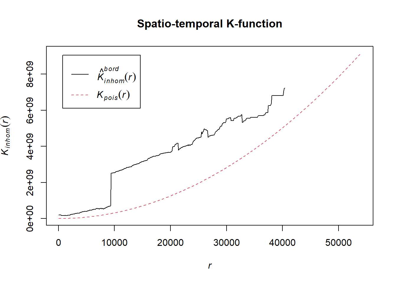
# Perform the CSR test with 99 simulations
K_ck.csr <- envelope(acled_spatio_ppp_owin, Kinhom, nsim=99, correction="border", parallel = parallel::detectCores())Generating 99 simulations of CSR ...
1, 2, 3, 4, 5, 6, 7, 8, 9, 10, 11, 12, 13, 14, 15, 16, 17, 18, 19, 20,
21, 22, 23, 24, 25, 26, 27, 28, 29, 30, 31, 32, 33, 34, 35, 36, 37, 38, 39, 40,
41, 42, 43, 44, 45, 46, 47, 48, 49, 50, 51, 52, 53, 54, 55, 56, 57, 58, 59, 60,
61, 62, 63, 64, 65, 66, 67, 68, 69, 70, 71, 72, 73, 74, 75, 76, 77, 78, 79, 80,
81, 82, 83, 84, 85, 86, 87, 88, 89, 90, 91, 92, 93, 94, 95, 96, 97, 98,
99.
Done.# Plot the envelope with the observed K-function
plot(K_ck.csr, main="Spatio-temporal K-function Envelope", legend=TRUE)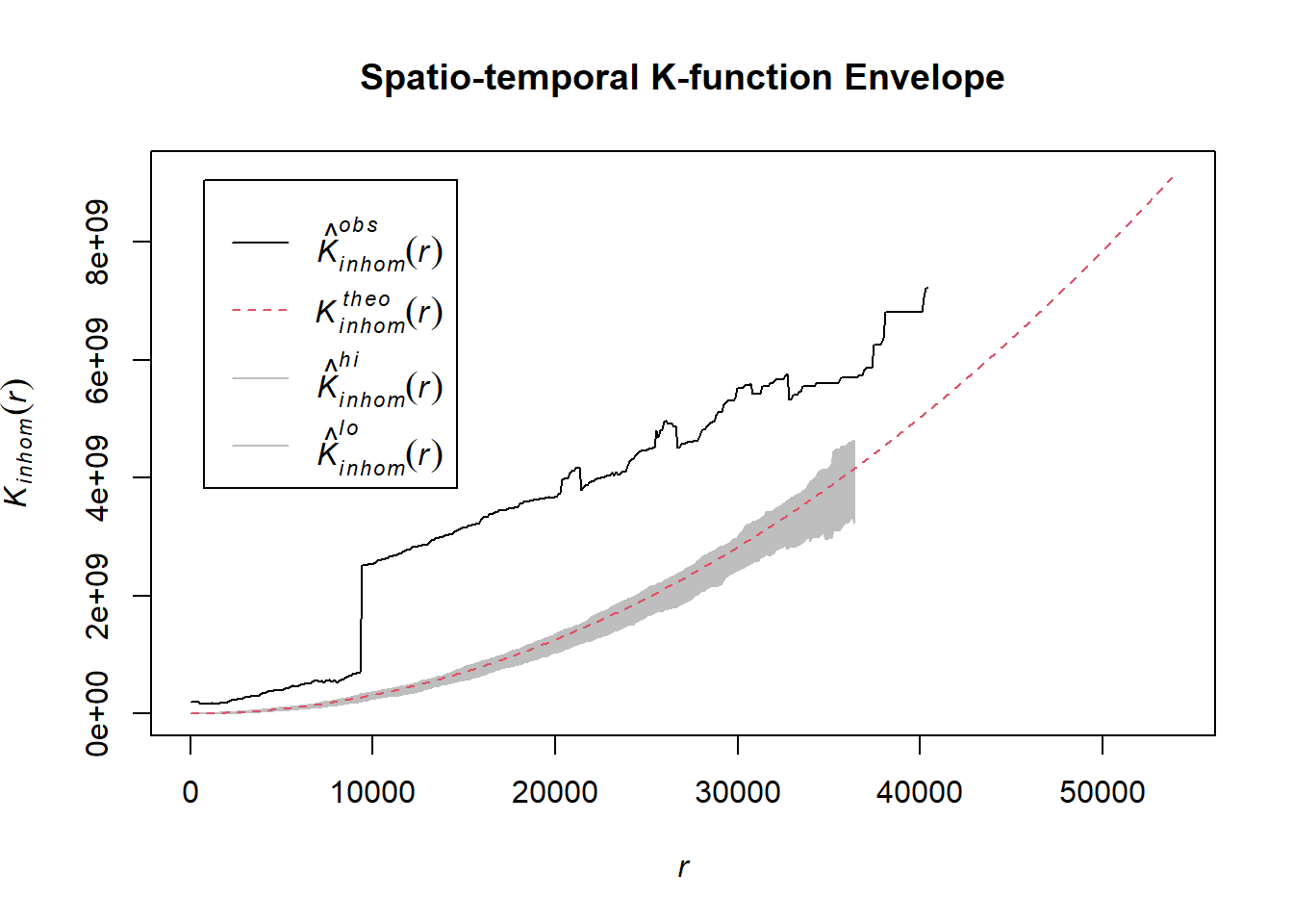
# Assuming `acled_spatio_ppp_owin` is your spatio-temporal point pattern object:
acled_spatio_ppp_owin <- mandalay_acled_quarters_2024_ppp[mandalay_owin]
K_st <- Kinhom(acled_spatio_ppp_owin, correction="border")
# Plot the result for visual inspection
plot(K_st, main = "Spatio-temporal K-function", legend=TRUE)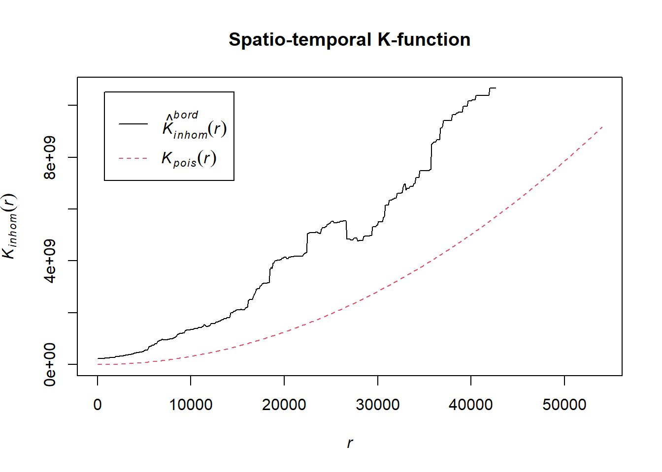
# Perform the CSR test with 99 simulations
K_ck.csr <- envelope(acled_spatio_ppp_owin, Kinhom, nsim=99, correction="border", parallel = parallel::detectCores())Generating 99 simulations of CSR ...
1, 2, 3, 4, 5, 6, 7, 8, 9, 10, 11, 12, 13, 14, 15, 16, 17, 18, 19, 20,
21, 22, 23, 24, 25, 26, 27, 28, 29, 30, 31, 32, 33, 34, 35, 36, 37, 38, 39, 40,
41, 42, 43, 44, 45, 46, 47, 48, 49, 50, 51, 52, 53, 54, 55, 56, 57, 58, 59, 60,
61, 62, 63, 64, 65, 66, 67, 68, 69, 70, 71, 72, 73, 74, 75, 76, 77, 78, 79, 80,
81, 82, 83, 84, 85, 86, 87, 88, 89, 90, 91, 92, 93, 94, 95, 96, 97, 98,
99.
Done.# Plot the envelope with the observed K-function
plot(K_ck.csr, main="Spatio-temporal K-function Envelope", legend=TRUE)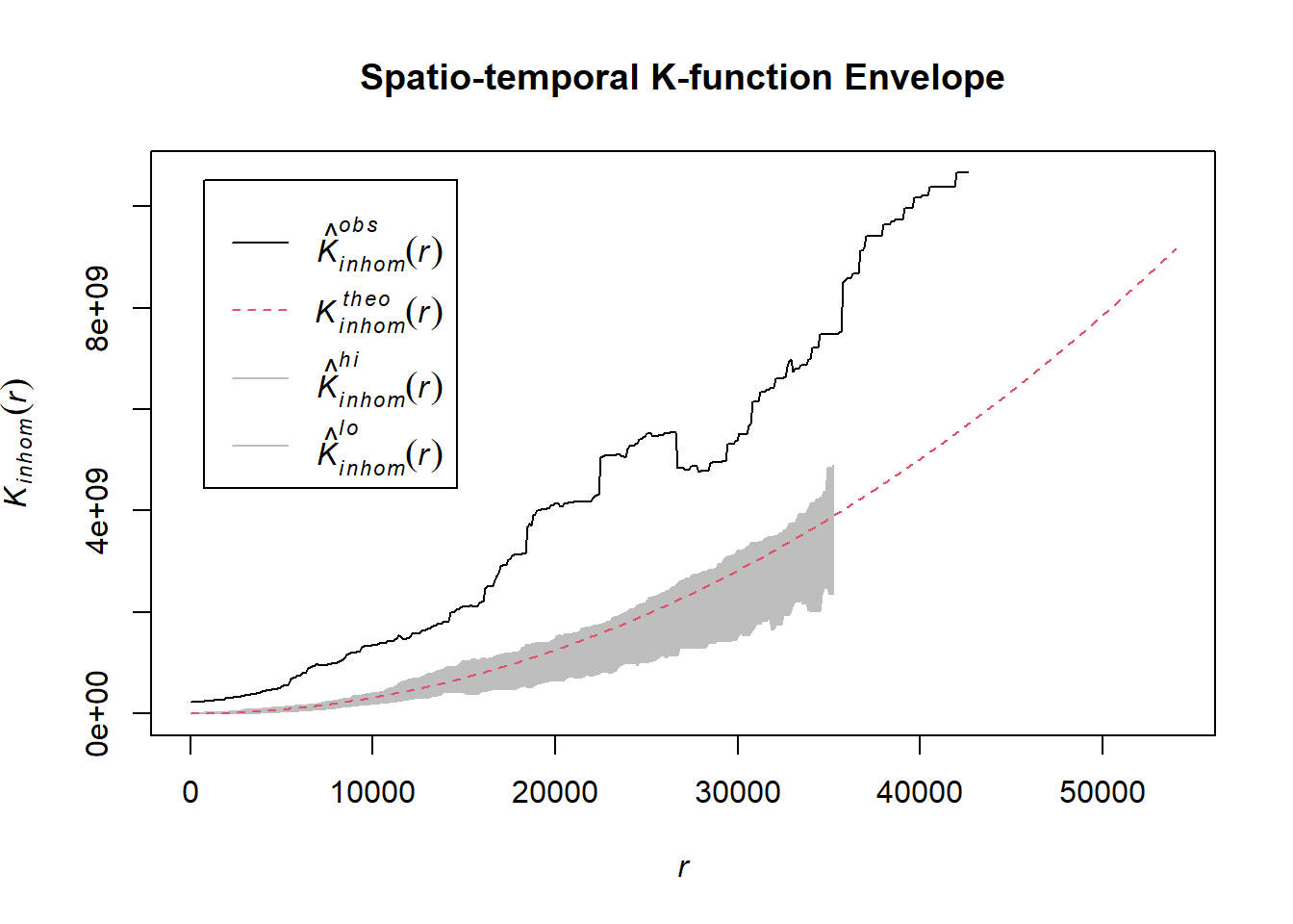
1.8.4.4.2 Strategic developments
Example <- "Strategic developments"
mandalay_acled_quarters_2021_ppp <- as.ppp(mandalay_acled_sf %>%
filter(year == 2021 & event_type == Example) %>%
select(q))
mandalay_acled_quarters_2022_ppp <- as.ppp(mandalay_acled_sf %>%
filter(year == 2022 & event_type == Example) %>%
select(q))
mandalay_acled_quarters_2023_ppp <- as.ppp(mandalay_acled_sf %>%
filter(year == 2023 & event_type == Example) %>%
select(q))
mandalay_acled_quarters_2024_ppp <- as.ppp(mandalay_acled_sf %>%
filter(year == 2024 & event_type == Example) %>%
select(q))# Assuming `acled_spatio_ppp_owin` is your spatio-temporal point pattern object:
acled_spatio_ppp_owin <- mandalay_acled_quarters_2021_ppp[mandalay_owin]
K_st <- Kinhom(acled_spatio_ppp_owin, correction="border")
# Plot the result for visual inspection
plot(K_st, main = "Spatio-temporal K-function", legend=TRUE)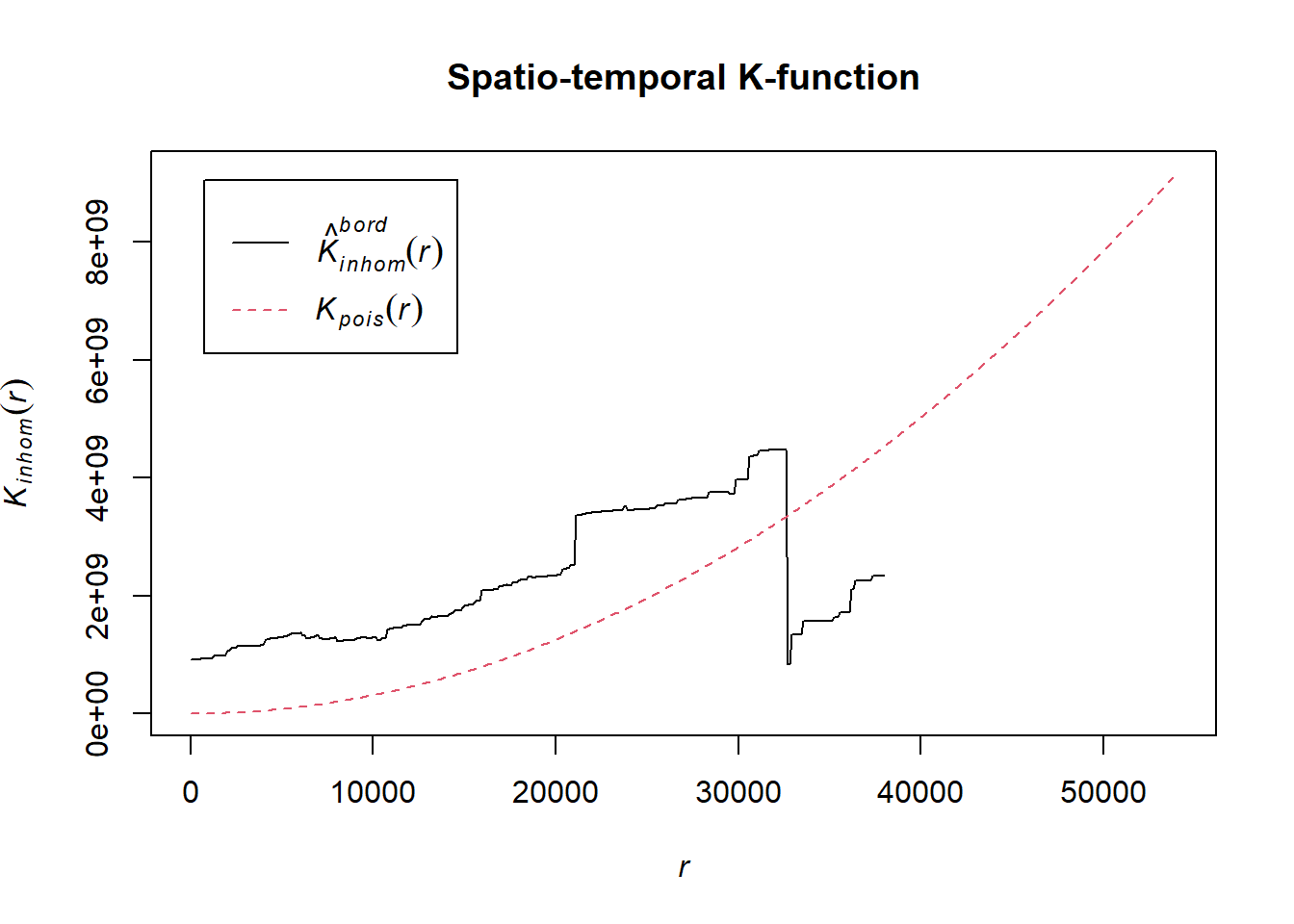
# Perform the CSR test with 99 simulations
K_ck.csr <- envelope(acled_spatio_ppp_owin, Kinhom, nsim=99, correction="border", parallel = parallel::detectCores())Generating 99 simulations of CSR ...
1, 2, 3, 4, 5, 6, 7, 8, 9, 10, 11, 12, 13, 14, 15, 16, 17, 18, 19, 20,
21, 22, 23, 24, 25, 26, 27, 28, 29, 30, 31, 32, 33, 34, 35, 36, 37, 38, 39, 40,
41, 42, 43, 44, 45, 46, 47, 48, 49, 50, 51, 52, 53, 54, 55, 56, 57, 58, 59, 60,
61, 62, 63, 64, 65, 66, 67, 68, 69, 70, 71, 72, 73, 74, 75, 76, 77, 78, 79, 80,
81, 82, 83, 84, 85, 86, 87, 88, 89, 90, 91, 92, 93, 94, 95, 96, 97, 98,
99.
Done.# Plot the envelope with the observed K-function
plot(K_ck.csr, main="Spatio-temporal K-function Envelope", legend=TRUE)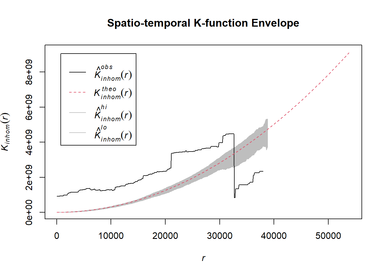
# Assuming `acled_spatio_ppp_owin` is your spatio-temporal point pattern object:
acled_spatio_ppp_owin <- mandalay_acled_quarters_2022_ppp[mandalay_owin]
K_st <- Kinhom(acled_spatio_ppp_owin, correction="border")
# Plot the result for visual inspection
plot(K_st, main = "Spatio-temporal K-function", legend=TRUE)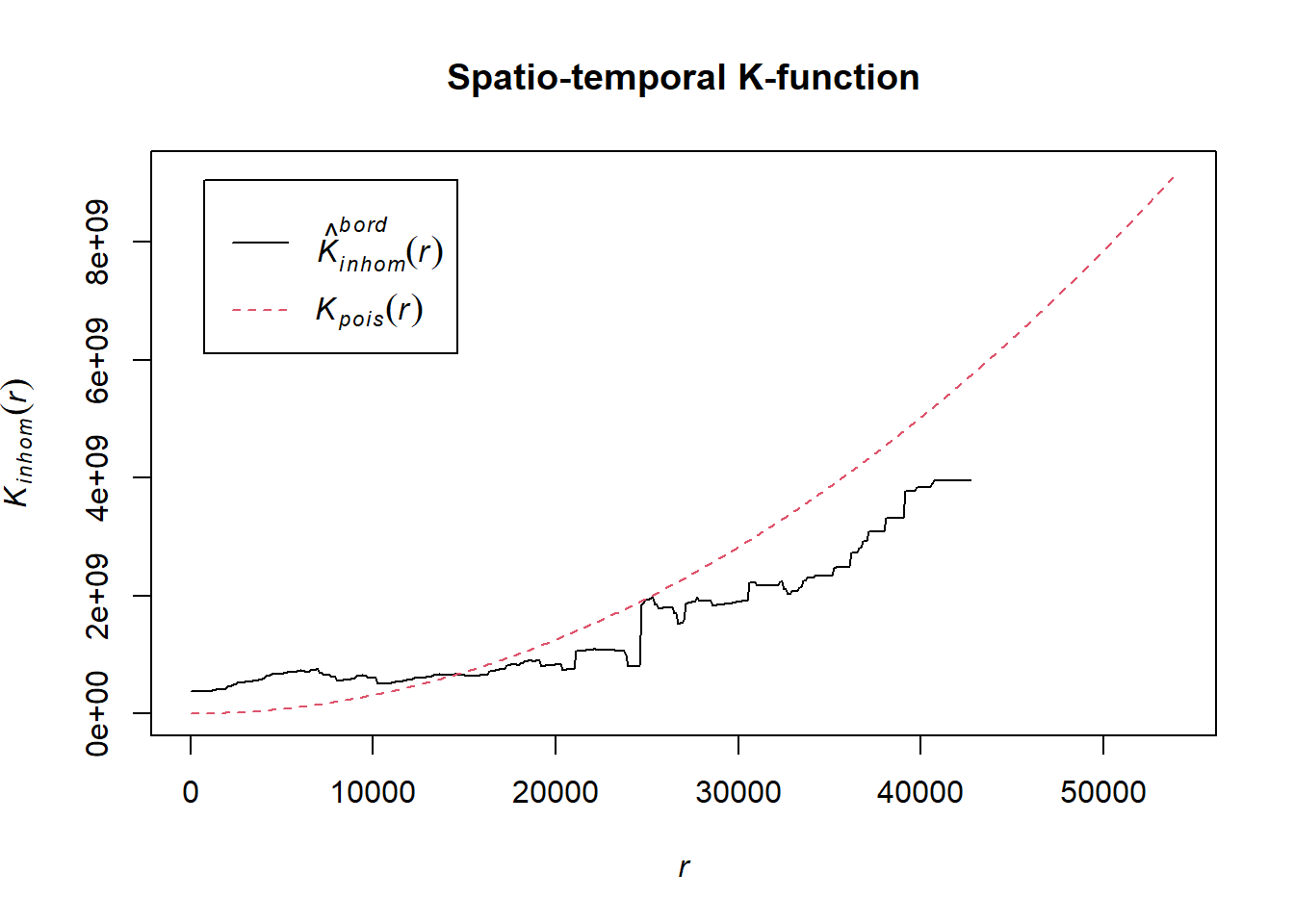
# Perform the CSR test with 99 simulations
K_ck.csr <- envelope(acled_spatio_ppp_owin, Kinhom, nsim=99, correction="border", parallel = parallel::detectCores())Generating 99 simulations of CSR ...
1, 2, 3, 4, 5, 6, 7, 8, 9, 10, 11, 12, 13, 14, 15, 16, 17, 18, 19, 20,
21, 22, 23, 24, 25, 26, 27, 28, 29, 30, 31, 32, 33, 34, 35, 36, 37, 38, 39, 40,
41, 42, 43, 44, 45, 46, 47, 48, 49, 50, 51, 52, 53, 54, 55, 56, 57, 58, 59, 60,
61, 62, 63, 64, 65, 66, 67, 68, 69, 70, 71, 72, 73, 74, 75, 76, 77, 78, 79, 80,
81, 82, 83, 84, 85, 86, 87, 88, 89, 90, 91, 92, 93, 94, 95, 96, 97, 98,
99.
Done.# Plot the envelope with the observed K-function
plot(K_ck.csr, main="Spatio-temporal K-function Envelope", legend=TRUE)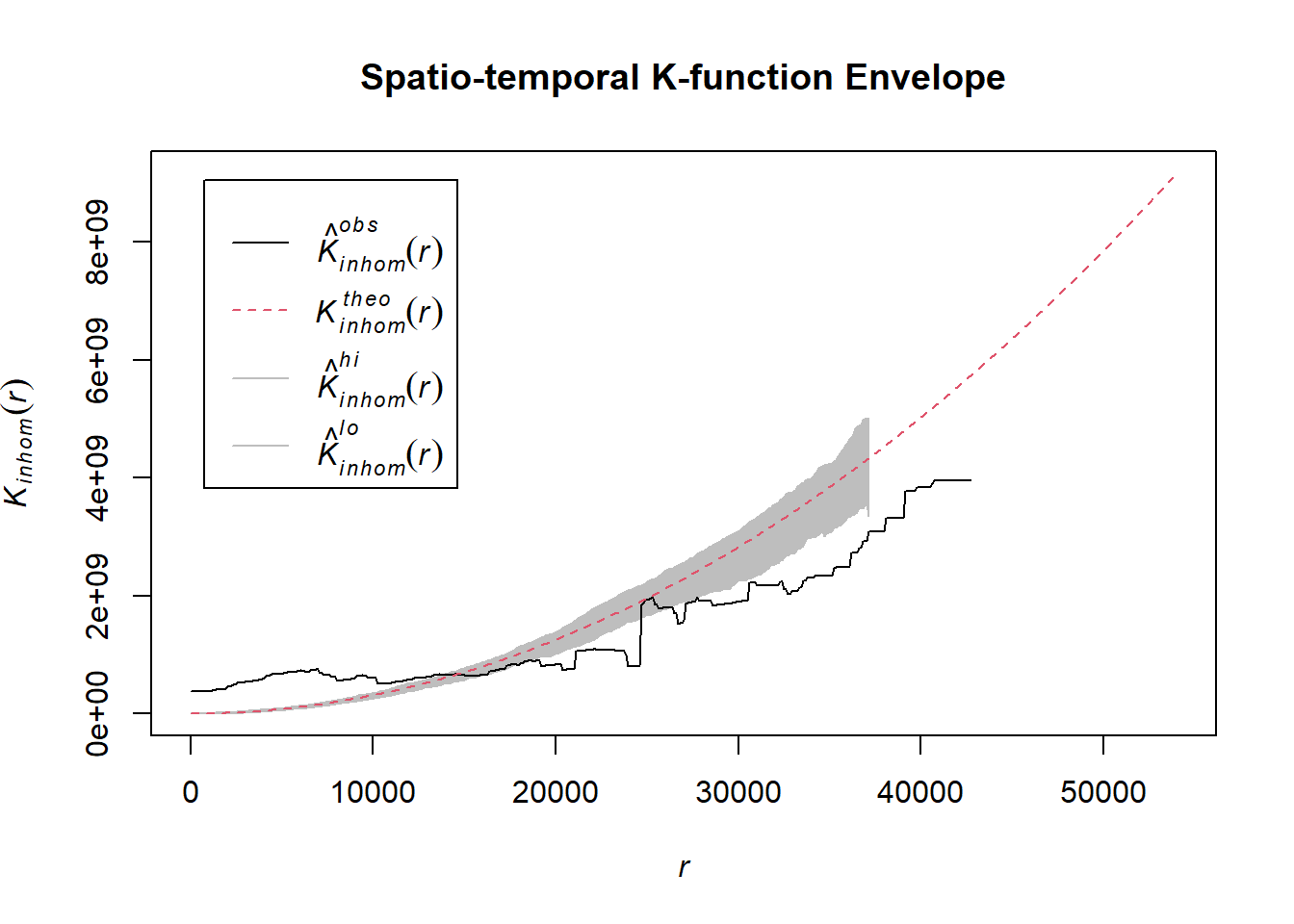
# Assuming `acled_spatio_ppp_owin` is your spatio-temporal point pattern object:
acled_spatio_ppp_owin <- mandalay_acled_quarters_2023_ppp[mandalay_owin]
K_st <- Kinhom(acled_spatio_ppp_owin, correction="border")
# Plot the result for visual inspection
plot(K_st, main = "Spatio-temporal K-function", legend=TRUE)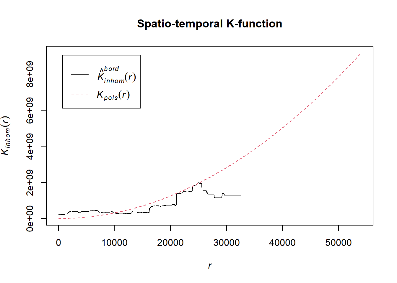
# Perform the CSR test with 99 simulations
K_ck.csr <- envelope(acled_spatio_ppp_owin, Kinhom, nsim=99, correction="border", parallel = parallel::detectCores())Generating 99 simulations of CSR ...
1, 2, 3, 4, 5, 6, 7, 8, 9, 10, 11, 12, 13, 14, 15, 16, 17, 18, 19, 20,
21, 22, 23, 24, 25, 26, 27, 28, 29, 30, 31, 32, 33, 34, 35, 36, 37, 38, 39, 40,
41, 42, 43, 44, 45, 46, 47, 48, 49, 50, 51, 52, 53, 54, 55, 56, 57, 58, 59, 60,
61, 62, 63, 64, 65, 66, 67, 68, 69, 70, 71, 72, 73, 74, 75, 76, 77, 78, 79, 80,
81, 82, 83, 84, 85, 86, 87, 88, 89, 90, 91, 92, 93, 94, 95, 96, 97, 98,
99.
Done.# Plot the envelope with the observed K-function
plot(K_ck.csr, main="Spatio-temporal K-function Envelope", legend=TRUE)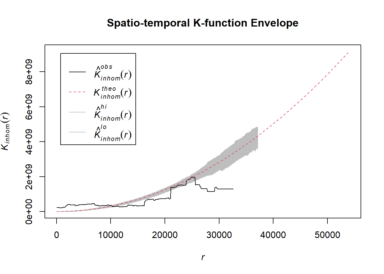
# Assuming `acled_spatio_ppp_owin` is your spatio-temporal point pattern object:
acled_spatio_ppp_owin <- mandalay_acled_quarters_2024_ppp[mandalay_owin]
K_st <- Kinhom(acled_spatio_ppp_owin, correction="border")
# Plot the result for visual inspection
plot(K_st, main = "Spatio-temporal K-function", legend=TRUE)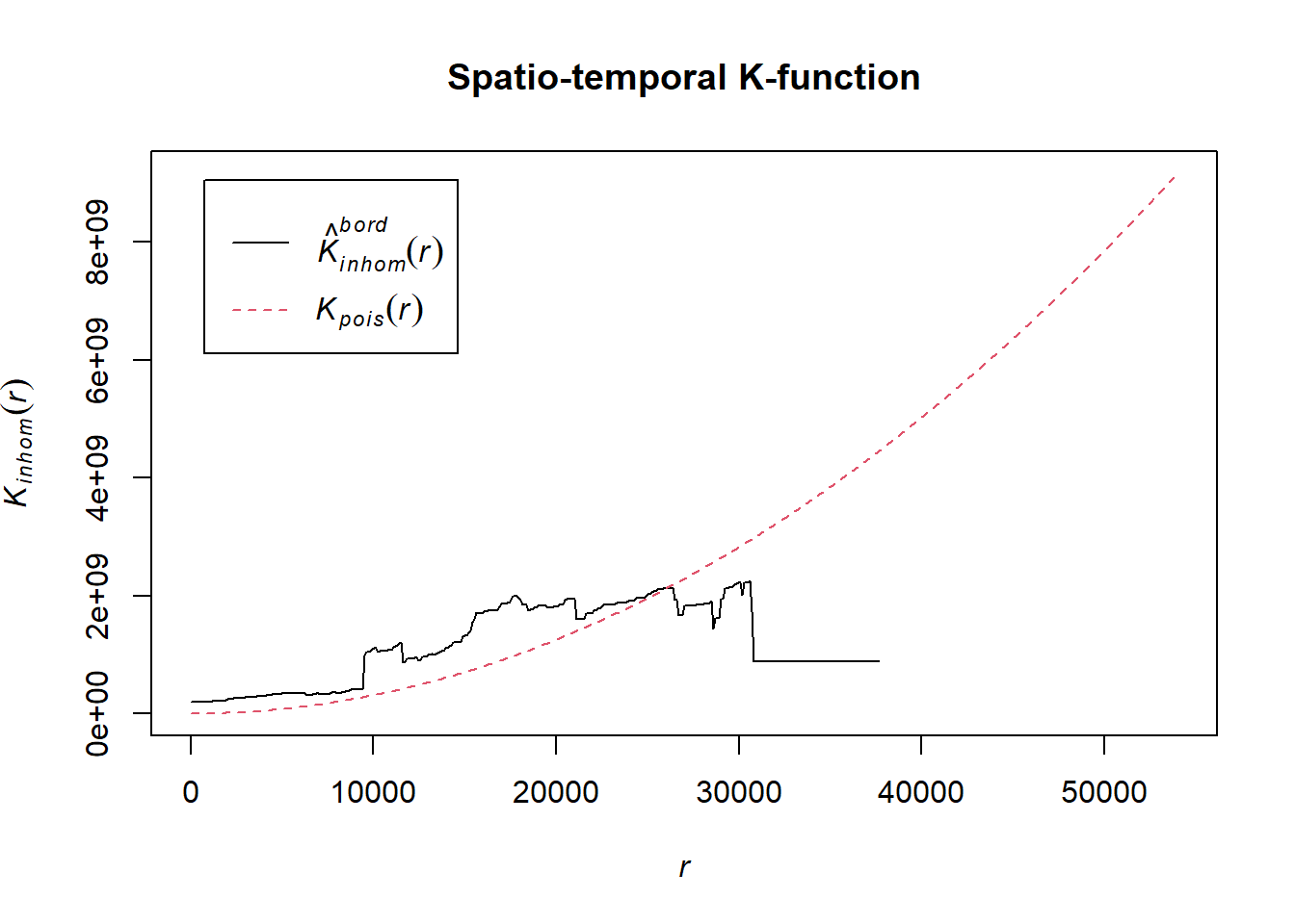
# Perform the CSR test with 99 simulations
K_ck.csr <- envelope(acled_spatio_ppp_owin, Kinhom, nsim=99, correction="border", parallel = parallel::detectCores())Generating 99 simulations of CSR ...
1, 2, 3, 4, 5, 6, 7, 8, 9, 10, 11, 12, 13, 14, 15, 16, 17, 18, 19, 20,
21, 22, 23, 24, 25, 26, 27, 28, 29, 30, 31, 32, 33, 34, 35, 36, 37, 38, 39, 40,
41, 42, 43, 44, 45, 46, 47, 48, 49, 50, 51, 52, 53, 54, 55, 56, 57, 58, 59, 60,
61, 62, 63, 64, 65, 66, 67, 68, 69, 70, 71, 72, 73, 74, 75, 76, 77, 78, 79, 80,
81, 82, 83, 84, 85, 86, 87, 88, 89, 90, 91, 92, 93, 94, 95, 96, 97, 98,
99.
Done.# Plot the envelope with the observed K-function
plot(K_ck.csr, main="Spatio-temporal K-function Envelope", legend=TRUE)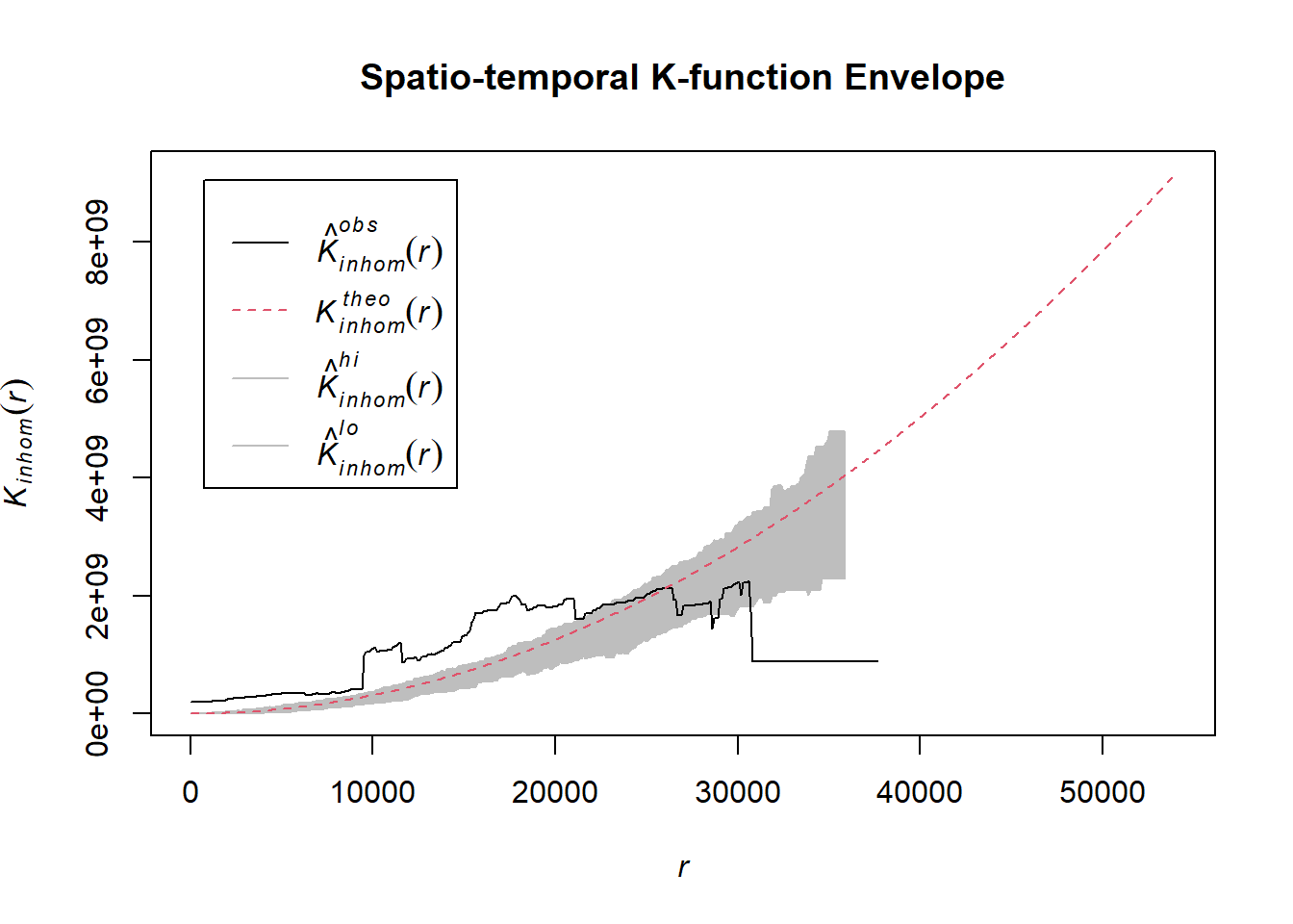
1.8.4.4.3 Battles
Example <- "Battles"
mandalay_acled_quarters_2021_ppp <- as.ppp(mandalay_acled_sf %>%
filter(year == 2021 & event_type == Example) %>%
select(q))
mandalay_acled_quarters_2022_ppp <- as.ppp(mandalay_acled_sf %>%
filter(year == 2022 & event_type == Example) %>%
select(q))
mandalay_acled_quarters_2023_ppp <- as.ppp(mandalay_acled_sf %>%
filter(year == 2023 & event_type == Example) %>%
select(q))
mandalay_acled_quarters_2024_ppp <- as.ppp(mandalay_acled_sf %>%
filter(year == 2024 & event_type == Example) %>%
select(q))# Assuming `acled_spatio_ppp_owin` is your spatio-temporal point pattern object:
acled_spatio_ppp_owin <- mandalay_acled_quarters_2021_ppp[mandalay_owin]
K_st <- Kinhom(acled_spatio_ppp_owin, correction="border")
# Plot the result for visual inspection
plot(K_st, main = "Spatio-temporal K-function", legend=TRUE)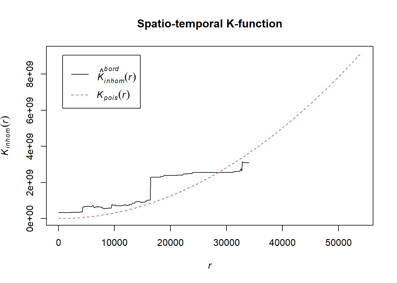
# Perform the CSR test with 99 simulations
K_ck.csr <- envelope(acled_spatio_ppp_owin, Kinhom, nsim=99, correction="border", parallel = parallel::detectCores())Generating 99 simulations of CSR ...
1, 2, 3, 4, 5, 6, 7, 8, 9, 10, 11, 12, 13, 14, 15, 16, 17, 18, 19, 20,
21, 22, 23, 24, 25, 26, 27, 28, 29, 30, 31, 32, 33, 34, 35, 36, 37, 38, 39, 40,
41, 42, 43, 44, 45, 46, 47, 48, 49, 50, 51, 52, 53, 54, 55, 56, 57, 58, 59, 60,
61, 62, 63, 64, 65, 66, 67, 68, 69, 70, 71, 72, 73, 74, 75, 76, 77, 78, 79, 80,
81, 82, 83, 84, 85, 86, 87, 88, 89, 90, 91, 92, 93, 94, 95, 96, 97, 98,
99.
Done.# Plot the envelope with the observed K-function
plot(K_ck.csr, main="Spatio-temporal K-function Envelope", legend=TRUE)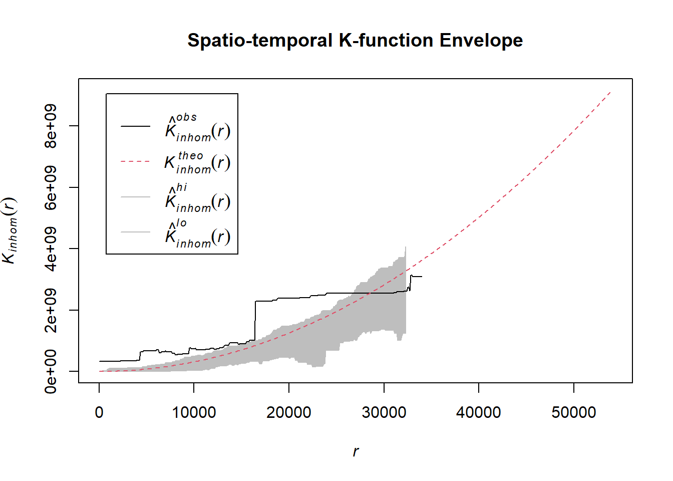
# Assuming `acled_spatio_ppp_owin` is your spatio-temporal point pattern object:
acled_spatio_ppp_owin <- mandalay_acled_quarters_2022_ppp[mandalay_owin]
K_st <- Kinhom(acled_spatio_ppp_owin, correction="border")
# Plot the result for visual inspection
plot(K_st, main = "Spatio-temporal K-function", legend=TRUE)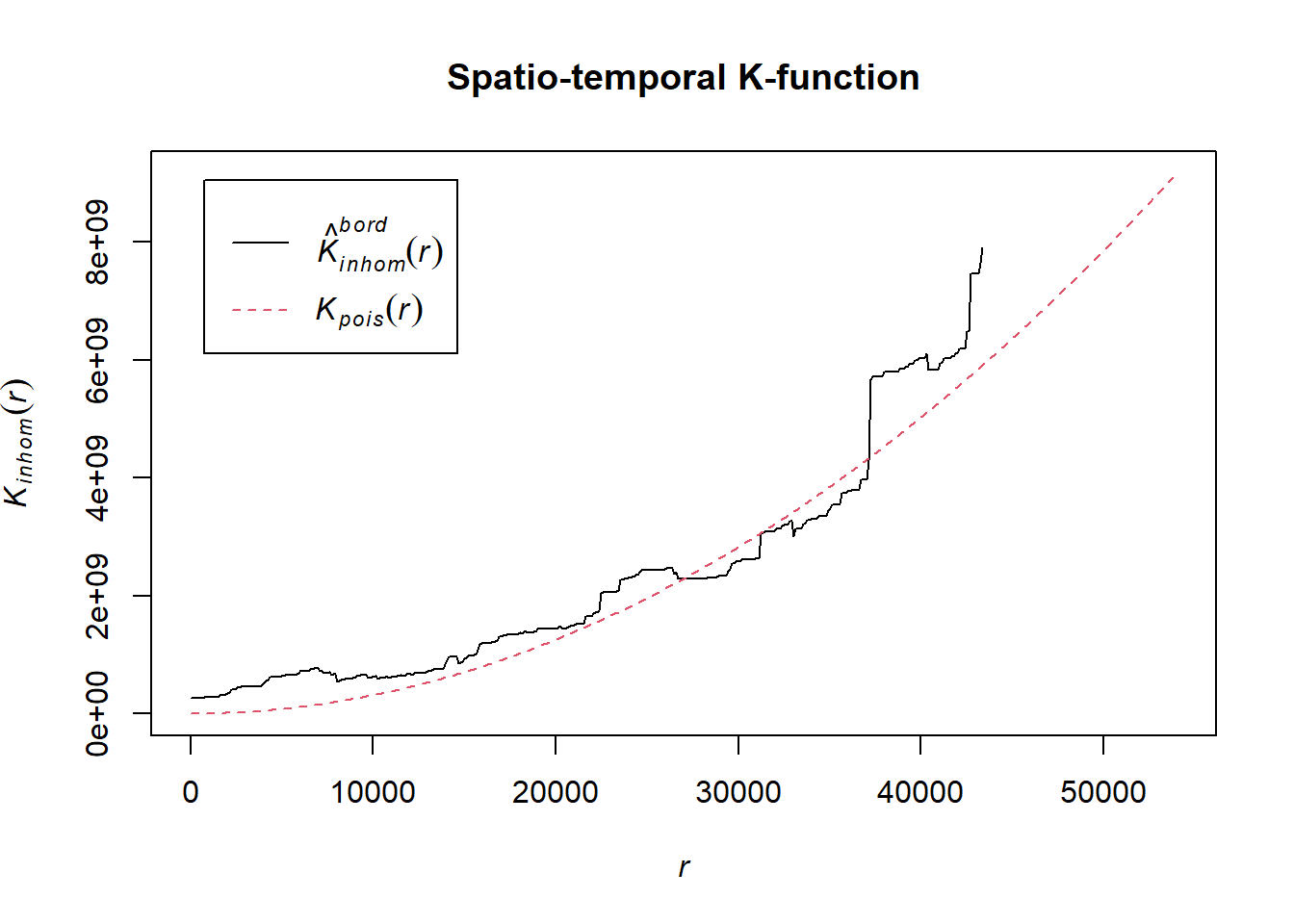
# Perform the CSR test with 99 simulations
K_ck.csr <- envelope(acled_spatio_ppp_owin, Kinhom, nsim=99, correction="border", parallel = parallel::detectCores())Generating 99 simulations of CSR ...
1, 2, 3, 4, 5, 6, 7, 8, 9, 10, 11, 12, 13, 14, 15, 16, 17, 18, 19, 20,
21, 22, 23, 24, 25, 26, 27, 28, 29, 30, 31, 32, 33, 34, 35, 36, 37, 38, 39, 40,
41, 42, 43, 44, 45, 46, 47, 48, 49, 50, 51, 52, 53, 54, 55, 56, 57, 58, 59, 60,
61, 62, 63, 64, 65, 66, 67, 68, 69, 70, 71, 72, 73, 74, 75, 76, 77, 78, 79, 80,
81, 82, 83, 84, 85, 86, 87, 88, 89, 90, 91, 92, 93, 94, 95, 96, 97, 98,
99.
Done.# Plot the envelope with the observed K-function
plot(K_ck.csr, main="Spatio-temporal K-function Envelope", legend=TRUE)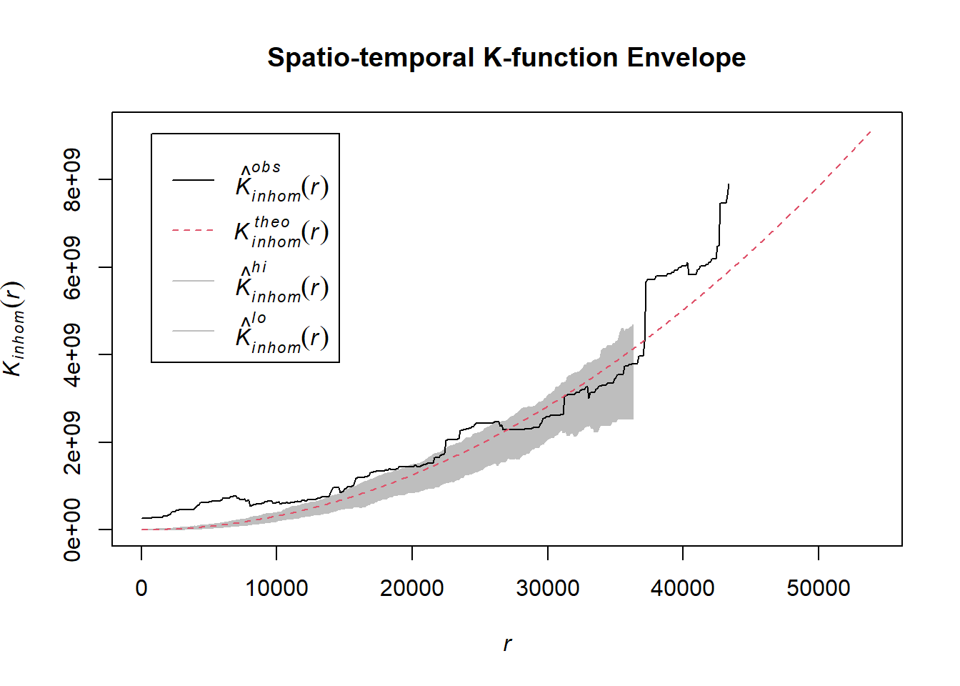
# Assuming `acled_spatio_ppp_owin` is your spatio-temporal point pattern object:
acled_spatio_ppp_owin <- mandalay_acled_quarters_2023_ppp[mandalay_owin]
K_st <- Kinhom(acled_spatio_ppp_owin, correction="border")
# Plot the result for visual inspection
plot(K_st, main = "Spatio-temporal K-function", legend=TRUE)
# Perform the CSR test with 99 simulations
K_ck.csr <- envelope(acled_spatio_ppp_owin, Kinhom, nsim=99, correction="border", parallel = parallel::detectCores())Generating 99 simulations of CSR ...
1, 2, 3, 4, 5, 6, 7, 8, 9, 10, 11, 12, 13, 14, 15, 16, 17, 18, 19, 20,
21, 22, 23, 24, 25, 26, 27, 28, 29, 30, 31, 32, 33, 34, 35, 36, 37, 38, 39, 40,
41, 42, 43, 44, 45, 46, 47, 48, 49, 50, 51, 52, 53, 54, 55, 56, 57, 58, 59, 60,
61, 62, 63, 64, 65, 66, 67, 68, 69, 70, 71, 72, 73, 74, 75, 76, 77, 78, 79, 80,
81, 82, 83, 84, 85, 86, 87, 88, 89, 90, 91, 92, 93, 94, 95, 96, 97, 98,
99.
Done.# Plot the envelope with the observed K-function
plot(K_ck.csr, main="Spatio-temporal K-function Envelope", legend=TRUE)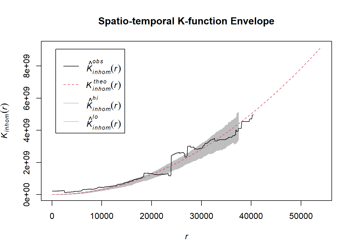
# Assuming `acled_spatio_ppp_owin` is your spatio-temporal point pattern object:
acled_spatio_ppp_owin <- mandalay_acled_quarters_2024_ppp[mandalay_owin]
K_st <- Kinhom(acled_spatio_ppp_owin, correction="border")
# Plot the result for visual inspection
plot(K_st, main = "Spatio-temporal K-function", legend=TRUE)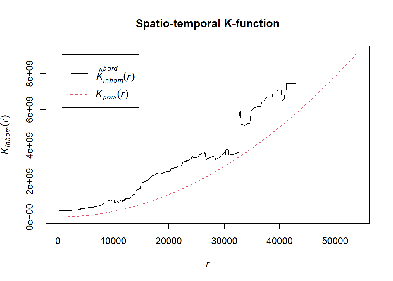
# Perform the CSR test with 99 simulations
K_ck.csr <- envelope(acled_spatio_ppp_owin, Kinhom, nsim=99, correction="border", parallel = parallel::detectCores())Generating 99 simulations of CSR ...
1, 2, 3, 4, 5, 6, 7, 8, 9, 10, 11, 12, 13, 14, 15, 16, 17, 18, 19, 20,
21, 22, 23, 24, 25, 26, 27, 28, 29, 30, 31, 32, 33, 34, 35, 36, 37, 38, 39, 40,
41, 42, 43, 44, 45, 46, 47, 48, 49, 50, 51, 52, 53, 54, 55, 56, 57, 58, 59, 60,
61, 62, 63, 64, 65, 66, 67, 68, 69, 70, 71, 72, 73, 74, 75, 76, 77, 78, 79, 80,
81, 82, 83, 84, 85, 86, 87, 88, 89, 90, 91, 92, 93, 94, 95, 96, 97, 98,
99.
Done.# Plot the envelope with the observed K-function
plot(K_ck.csr, main="Spatio-temporal K-function Envelope", legend=TRUE)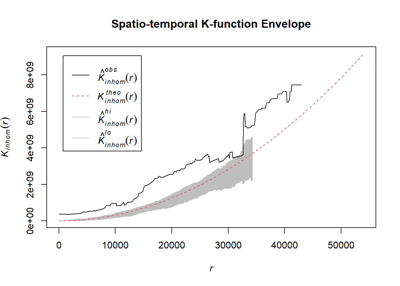
1.8.4.4.4 Violence against civilians
Example <- "Violence against civilians"
acled_quarters_2021_ppp <- as.ppp(temporal_acled_sf %>%
filter(year == 2021 & event_type == Example) %>%
select(q))
acled_quarters_2022_ppp <- as.ppp(temporal_acled_sf %>%
filter(year == 2022 & event_type == Example) %>%
select(q))
acled_quarters_2023_ppp <- as.ppp(temporal_acled_sf %>%
filter(year == 2023 & event_type == Example) %>%
select(q))
acled_quarters_2024_ppp <- as.ppp(temporal_acled_sf %>%
filter(year == 2024 & event_type == Example) %>%
select(q))# Assuming `acled_spatio_ppp_owin` is your spatio-temporal point pattern object:
acled_spatio_ppp_owin <- mandalay_acled_quarters_2021_ppp[mandalay_owin]
K_st <- Kinhom(acled_spatio_ppp_owin, correction="border")
# Plot the result for visual inspection
plot(K_st, main = "Spatio-temporal K-function", legend=TRUE)
# Perform the CSR test with 99 simulations
K_ck.csr <- envelope(acled_spatio_ppp_owin, Kinhom, nsim=99, correction="border", parallel = parallel::detectCores())Generating 99 simulations of CSR ...
1, 2, 3, 4, 5, 6, 7, 8, 9, 10, 11, 12, 13, 14, 15, 16, 17, 18, 19, 20,
21, 22, 23, 24, 25, 26, 27, 28, 29, 30, 31, 32, 33, 34, 35, 36, 37, 38, 39, 40,
41, 42, 43, 44, 45, 46, 47, 48, 49, 50, 51, 52, 53, 54, 55, 56, 57, 58, 59, 60,
61, 62, 63, 64, 65, 66, 67, 68, 69, 70, 71, 72, 73, 74, 75, 76, 77, 78, 79, 80,
81, 82, 83, 84, 85, 86, 87, 88, 89, 90, 91, 92, 93, 94, 95, 96, 97, 98,
99.
Done.# Plot the envelope with the observed K-function
plot(K_ck.csr, main="Spatio-temporal K-function Envelope", legend=TRUE)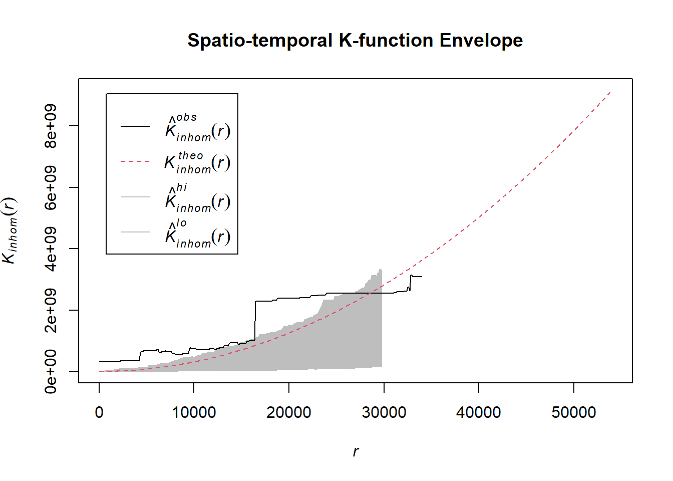
# Assuming `acled_spatio_ppp_owin` is your spatio-temporal point pattern object:
acled_spatio_ppp_owin <- mandalay_acled_quarters_2022_ppp[mandalay_owin]
K_st <- Kinhom(acled_spatio_ppp_owin, correction="border")
# Plot the result for visual inspection
plot(K_st, main = "Spatio-temporal K-function", legend=TRUE)
# Perform the CSR test with 99 simulations
K_ck.csr <- envelope(acled_spatio_ppp_owin, Kinhom, nsim=99, correction="border", parallel = parallel::detectCores())Generating 99 simulations of CSR ...
1, 2, 3, 4, 5, 6, 7, 8, 9, 10, 11, 12, 13, 14, 15, 16, 17, 18, 19, 20,
21, 22, 23, 24, 25, 26, 27, 28, 29, 30, 31, 32, 33, 34, 35, 36, 37, 38, 39, 40,
41, 42, 43, 44, 45, 46, 47, 48, 49, 50, 51, 52, 53, 54, 55, 56, 57, 58, 59, 60,
61, 62, 63, 64, 65, 66, 67, 68, 69, 70, 71, 72, 73, 74, 75, 76, 77, 78, 79, 80,
81, 82, 83, 84, 85, 86, 87, 88, 89, 90, 91, 92, 93, 94, 95, 96, 97, 98,
99.
Done.# Plot the envelope with the observed K-function
plot(K_ck.csr, main="Spatio-temporal K-function Envelope", legend=TRUE)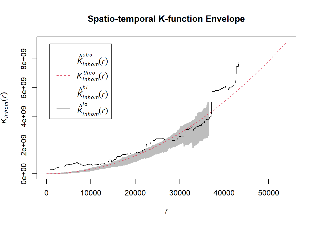
# Assuming `acled_spatio_ppp_owin` is your spatio-temporal point pattern object:
acled_spatio_ppp_owin <- mandalay_acled_quarters_2023_ppp[mandalay_owin]
K_st <- Kinhom(acled_spatio_ppp_owin, correction="border")
# Plot the result for visual inspection
plot(K_st, main = "Spatio-temporal K-function", legend=TRUE)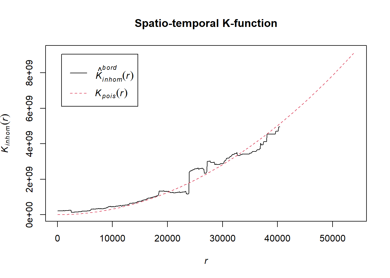
# Perform the CSR test with 99 simulations
K_ck.csr <- envelope(acled_spatio_ppp_owin, Kinhom, nsim=99, correction="border", parallel = parallel::detectCores())Generating 99 simulations of CSR ...
1, 2, 3, 4, 5, 6, 7, 8, 9, 10, 11, 12, 13, 14, 15, 16, 17, 18, 19, 20,
21, 22, 23, 24, 25, 26, 27, 28, 29, 30, 31, 32, 33, 34, 35, 36, 37, 38, 39, 40,
41, 42, 43, 44, 45, 46, 47, 48, 49, 50, 51, 52, 53, 54, 55, 56, 57, 58, 59, 60,
61, 62, 63, 64, 65, 66, 67, 68, 69, 70, 71, 72, 73, 74, 75, 76, 77, 78, 79, 80,
81, 82, 83, 84, 85, 86, 87, 88, 89, 90, 91, 92, 93, 94, 95, 96, 97, 98,
99.
Done.# Plot the envelope with the observed K-function
plot(K_ck.csr, main="Spatio-temporal K-function Envelope", legend=TRUE)
# Assuming `acled_spatio_ppp_owin` is your spatio-temporal point pattern object:
acled_spatio_ppp_owin <- mandalay_acled_quarters_2024_ppp[mandalay_owin]
K_st <- Kinhom(acled_spatio_ppp_owin, correction="border")
# Plot the result for visual inspection
plot(K_st, main = "Spatio-temporal K-function", legend=TRUE)
# Perform the CSR test with 99 simulations
K_ck.csr <- envelope(acled_spatio_ppp_owin, Kinhom, nsim=99, correction="border", parallel = parallel::detectCores())Generating 99 simulations of CSR ...
1, 2, 3, 4, 5, 6, 7, 8, 9, 10, 11, 12, 13, 14, 15, 16, 17, 18, 19, 20,
21, 22, 23, 24, 25, 26, 27, 28, 29, 30, 31, 32, 33, 34, 35, 36, 37, 38, 39, 40,
41, 42, 43, 44, 45, 46, 47, 48, 49, 50, 51, 52, 53, 54, 55, 56, 57, 58, 59, 60,
61, 62, 63, 64, 65, 66, 67, 68, 69, 70, 71, 72, 73, 74, 75, 76, 77, 78, 79, 80,
81, 82, 83, 84, 85, 86, 87, 88, 89, 90, 91, 92, 93, 94, 95, 96, 97, 98,
99.
Done.# Plot the envelope with the observed K-function
plot(K_ck.csr, main="Spatio-temporal K-function Envelope", legend=TRUE)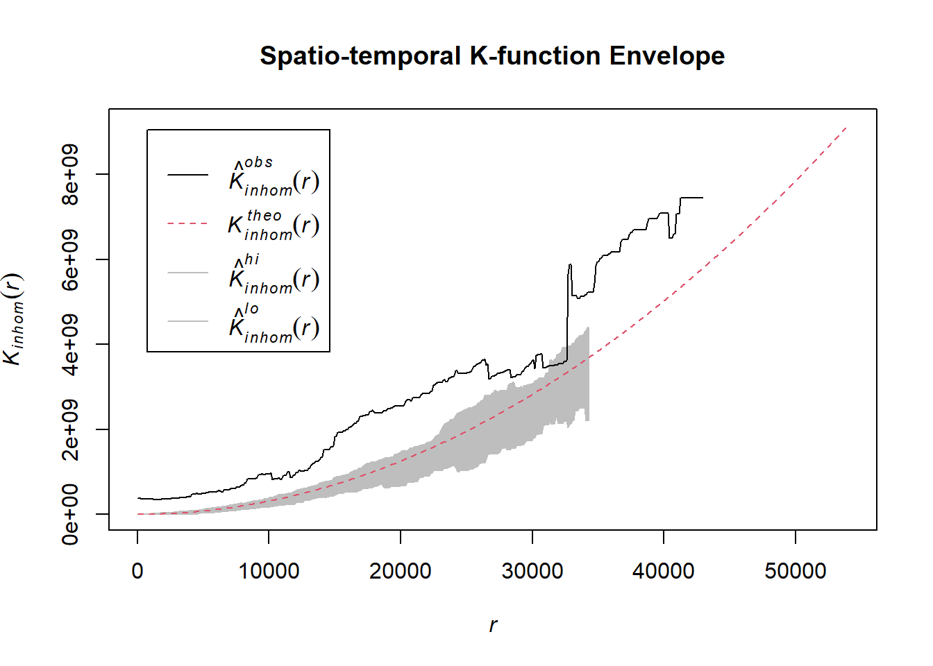
1.8.4.4 Magway Region
magway_acled_sf <- temporal_acled_sf %>% filter(admin1 == "Magway")
tm_shape(magway_sf)+
tm_polygons() +
tm_shape(magway_acled_sf) +
tm_dots(size=0.1) +
tm_facets(by="quarter",
free.coords=FALSE,
drop.units = TRUE) +
tm_layout(main.title = "Region and Boundaries of Magway",
main.title.position = "center",
main.title.size = 1,
legend.outside = TRUE,
frame = TRUE)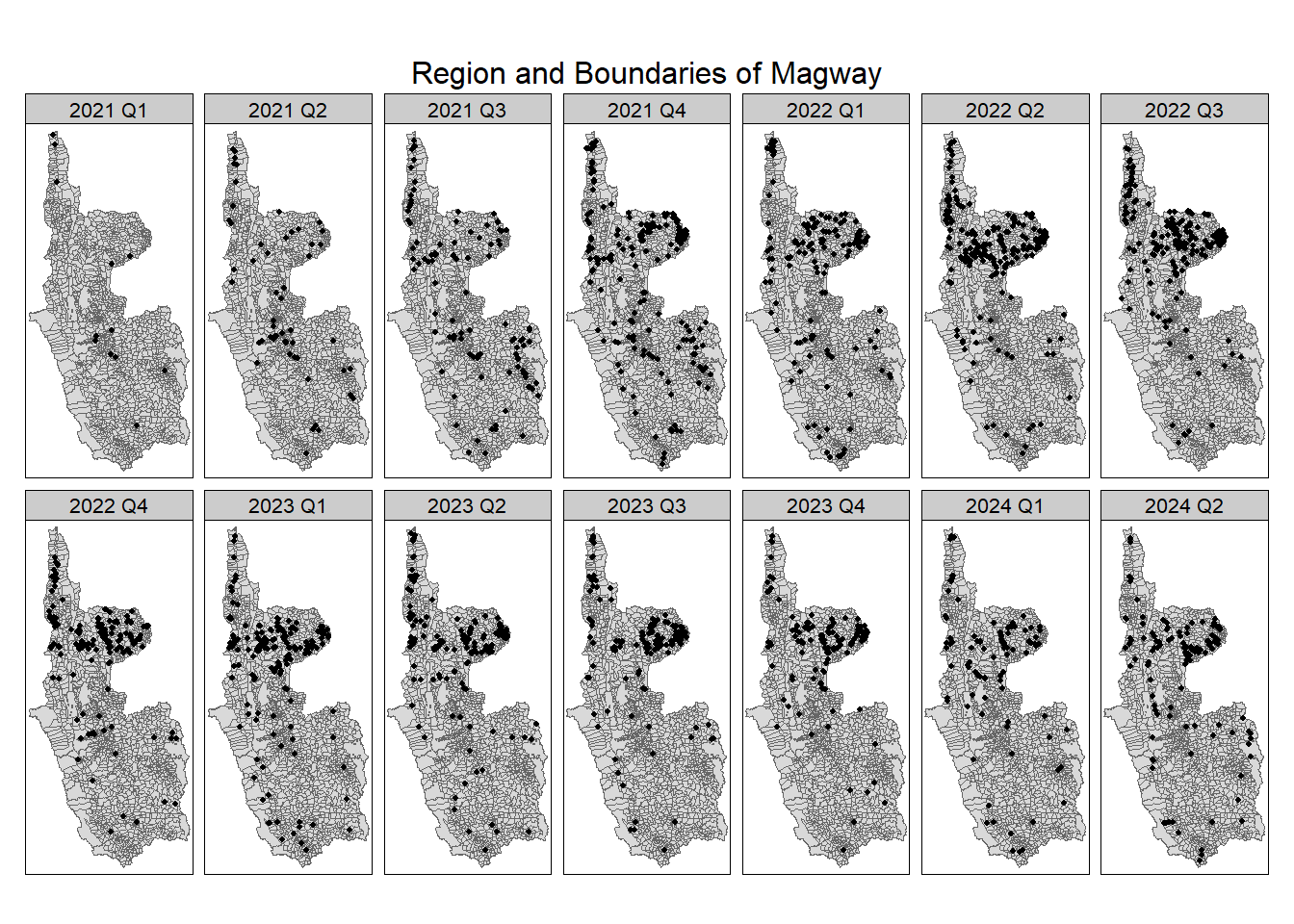
write_rds(magway_acled_sf, "data/rds/magway_acled_sf.rds")1.8.4.2.1 Explosions/Remote violence
Example <- "Explosions/Remote violence"
magway_acled_quarters_2021_ppp <- as.ppp(magway_acled_sf %>%
filter(year == 2021 & event_type == Example) %>%
select(q))
magway_acled_quarters_2022_ppp <- as.ppp(magway_acled_sf %>%
filter(year == 2022 & event_type == Example) %>%
select(q))
magway_acled_quarters_2023_ppp <- as.ppp(magway_acled_sf %>%
filter(year == 2023 & event_type == Example) %>%
select(q))
magway_acled_quarters_2024_ppp <- as.ppp(magway_acled_sf %>%
filter(year == 2024 & event_type == Example) %>%
select(q))# Assuming `acled_spatio_ppp_owin` is your spatio-temporal point pattern object:
acled_spatio_ppp_owin <- magway_acled_quarters_2021_ppp[magway_owin]
K_st <- Kinhom(acled_spatio_ppp_owin, correction="border")
# Plot the result for visual inspection
plot(K_st, main = "Spatio-temporal K-function", legend=TRUE)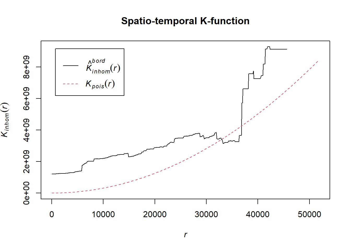
# Perform the CSR test with 99 simulations
K_ck.csr <- envelope(acled_spatio_ppp_owin, Kinhom, nsim=99, correction="border", parallel = parallel::detectCores())Generating 99 simulations of CSR ...
1, 2, 3, 4, 5, 6, 7, 8, 9, 10, 11, 12, 13, 14, 15, 16, 17, 18, 19, 20,
21, 22, 23, 24, 25, 26, 27, 28, 29, 30, 31, 32, 33, 34, 35, 36, 37, 38, 39, 40,
41, 42, 43, 44, 45, 46, 47, 48, 49, 50, 51, 52, 53, 54, 55, 56, 57, 58, 59, 60,
61, 62, 63, 64, 65, 66, 67, 68, 69, 70, 71, 72, 73, 74, 75, 76, 77, 78, 79, 80,
81, 82, 83, 84, 85, 86, 87, 88, 89, 90, 91, 92, 93, 94, 95, 96, 97, 98,
99.
Done.# Plot the envelope with the observed K-function
plot(K_ck.csr, main="Spatio-temporal K-function Envelope", legend=TRUE)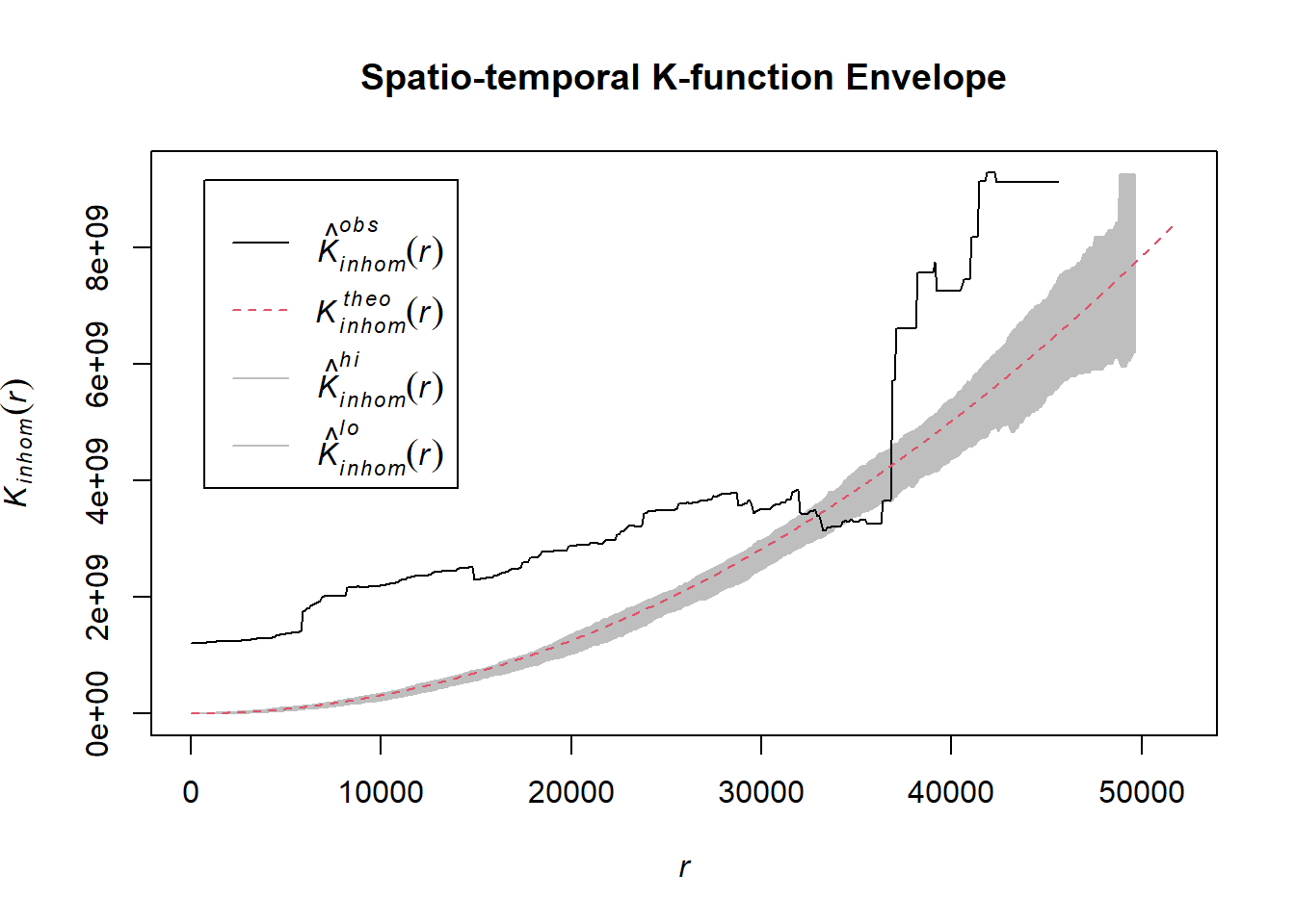
# Assuming `acled_spatio_ppp_owin` is your spatio-temporal point pattern object:
acled_spatio_ppp_owin <- magway_acled_quarters_2022_ppp[magway_owin]
K_st <- Kinhom(acled_spatio_ppp_owin, correction="border")
# Plot the result for visual inspection
plot(K_st, main = "Spatio-temporal K-function", legend=TRUE)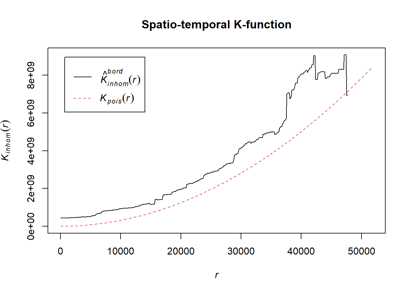
# Perform the CSR test with 99 simulations
K_ck.csr <- envelope(acled_spatio_ppp_owin, Kinhom, nsim=99, correction="border", parallel = parallel::detectCores())Generating 99 simulations of CSR ...
1, 2, 3, 4, 5, 6, 7, 8, 9, 10, 11, 12, 13, 14, 15, 16, 17, 18, 19, 20,
21, 22, 23, 24, 25, 26, 27, 28, 29, 30, 31, 32, 33, 34, 35, 36, 37, 38, 39, 40,
41, 42, 43, 44, 45, 46, 47, 48, 49, 50, 51, 52, 53, 54, 55, 56, 57, 58, 59, 60,
61, 62, 63, 64, 65, 66, 67, 68, 69, 70, 71, 72, 73, 74, 75, 76, 77, 78, 79, 80,
81, 82, 83, 84, 85, 86, 87, 88, 89, 90, 91, 92, 93, 94, 95, 96, 97, 98,
99.
Done.# Plot the envelope with the observed K-function
plot(K_ck.csr, main="Spatio-temporal K-function Envelope", legend=TRUE)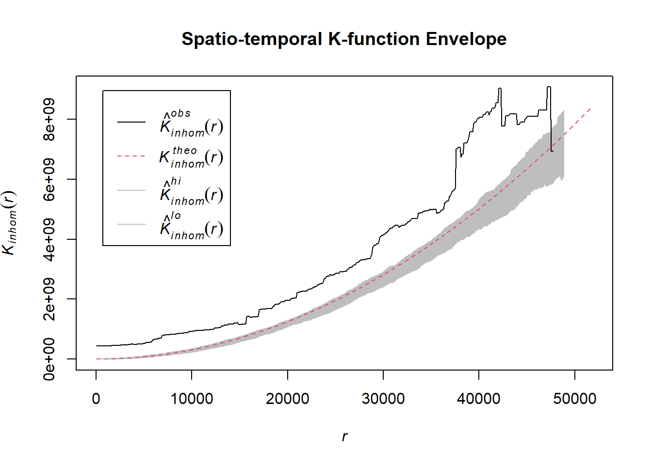
# Assuming `acled_spatio_ppp_owin` is your spatio-temporal point pattern object:
acled_spatio_ppp_owin <- magway_acled_quarters_2023_ppp[magway_owin]
K_st <- Kinhom(acled_spatio_ppp_owin, correction="border")
# Plot the result for visual inspection
plot(K_st, main = "Spatio-temporal K-function", legend=TRUE)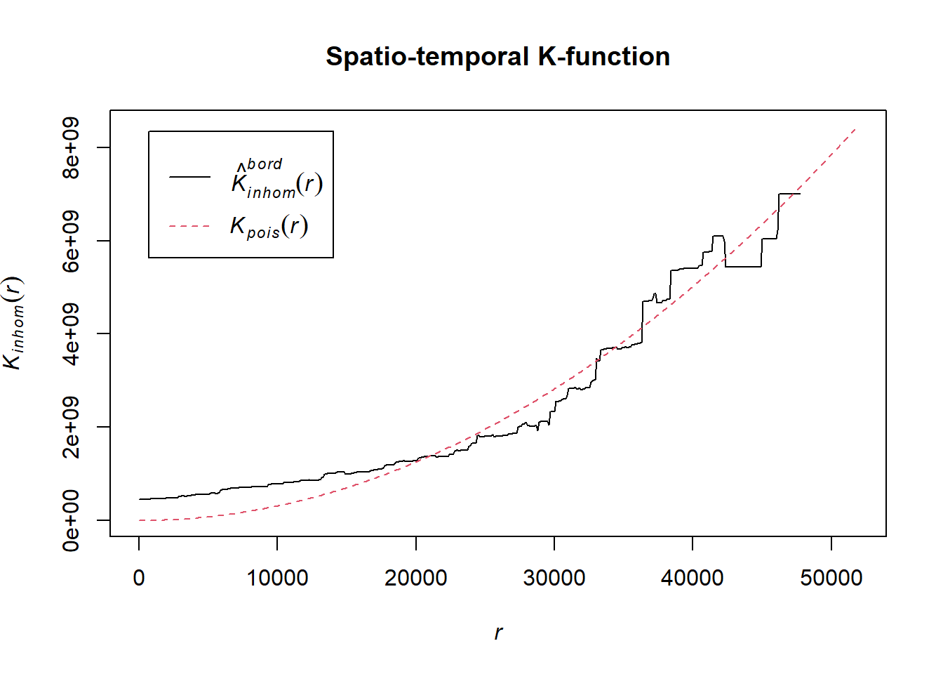
# Perform the CSR test with 99 simulations
K_ck.csr <- envelope(acled_spatio_ppp_owin, Kinhom, nsim=99, correction="border", parallel = parallel::detectCores())Generating 99 simulations of CSR ...
1, 2, 3, 4, 5, 6, 7, 8, 9, 10, 11, 12, 13, 14, 15, 16, 17, 18, 19, 20,
21, 22, 23, 24, 25, 26, 27, 28, 29, 30, 31, 32, 33, 34, 35, 36, 37, 38, 39, 40,
41, 42, 43, 44, 45, 46, 47, 48, 49, 50, 51, 52, 53, 54, 55, 56, 57, 58, 59, 60,
61, 62, 63, 64, 65, 66, 67, 68, 69, 70, 71, 72, 73, 74, 75, 76, 77, 78, 79, 80,
81, 82, 83, 84, 85, 86, 87, 88, 89, 90, 91, 92, 93, 94, 95, 96, 97, 98,
99.
Done.# Plot the envelope with the observed K-function
plot(K_ck.csr, main="Spatio-temporal K-function Envelope", legend=TRUE)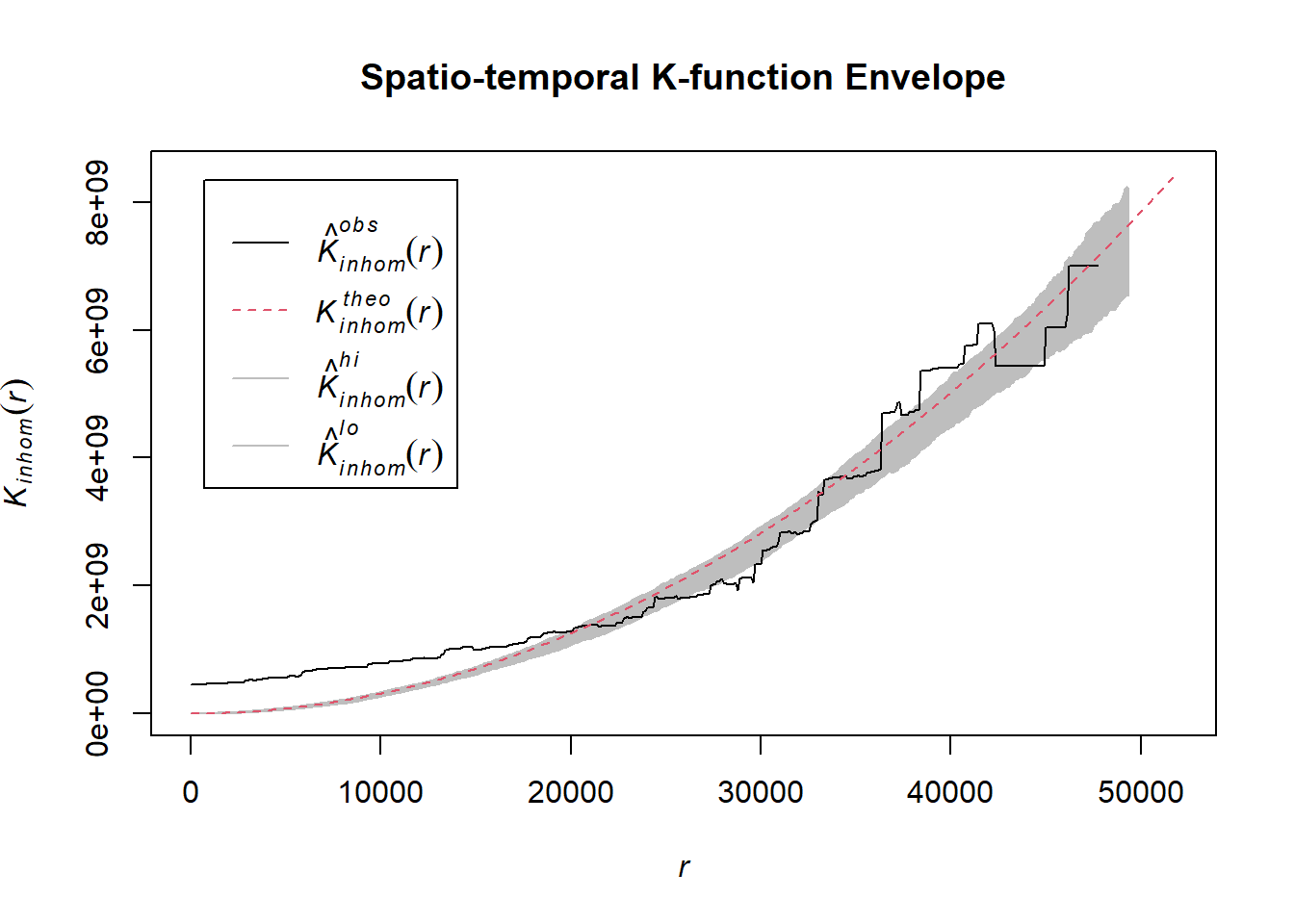
# Assuming `acled_spatio_ppp_owin` is your spatio-temporal point pattern object:
acled_spatio_ppp_owin <- magway_acled_quarters_2024_ppp[magway_owin]
K_st <- Kinhom(acled_spatio_ppp_owin, correction="border")
# Plot the result for visual inspection
plot(K_st, main = "Spatio-temporal K-function", legend=TRUE)
# Perform the CSR test with 99 simulations
K_ck.csr <- envelope(acled_spatio_ppp_owin, Kinhom, nsim=99, correction="border", parallel = parallel::detectCores())Generating 99 simulations of CSR ...
1, 2, 3, 4, 5, 6, 7, 8, 9, 10, 11, 12, 13, 14, 15, 16, 17, 18, 19, 20,
21, 22, 23, 24, 25, 26, 27, 28, 29, 30, 31, 32, 33, 34, 35, 36, 37, 38, 39, 40,
41, 42, 43, 44, 45, 46, 47, 48, 49, 50, 51, 52, 53, 54, 55, 56, 57, 58, 59, 60,
61, 62, 63, 64, 65, 66, 67, 68, 69, 70, 71, 72, 73, 74, 75, 76, 77, 78, 79, 80,
81, 82, 83, 84, 85, 86, 87, 88, 89, 90, 91, 92, 93, 94, 95, 96, 97, 98,
99.
Done.# Plot the envelope with the observed K-function
plot(K_ck.csr, main="Spatio-temporal K-function Envelope", legend=TRUE)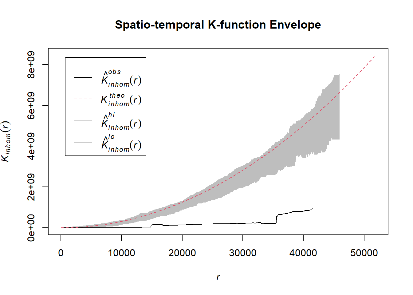
1.8.4.2.2 Strategic developments
Example <- "Strategic developments"
magway_acled_quarters_2021_ppp <- as.ppp(magway_acled_sf %>%
filter(year == 2021 & event_type == Example) %>%
select(q))
magway_acled_quarters_2022_ppp <- as.ppp(magway_acled_sf %>%
filter(year == 2022 & event_type == Example) %>%
select(q))
magway_acled_quarters_2023_ppp <- as.ppp(magway_acled_sf %>%
filter(year == 2023 & event_type == Example) %>%
select(q))
magway_acled_quarters_2024_ppp <- as.ppp(magway_acled_sf %>%
filter(year == 2024 & event_type == Example) %>%
select(q))# Assuming `acled_spatio_ppp_owin` is your spatio-temporal point pattern object:
acled_spatio_ppp_owin <- magway_acled_quarters_2021_ppp[magway_owin]
K_st <- Kinhom(acled_spatio_ppp_owin, correction="border")
# Plot the result for visual inspection
plot(K_st, main = "Spatio-temporal K-function", legend=TRUE)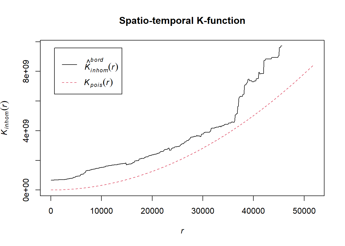
# Perform the CSR test with 99 simulations
K_ck.csr <- envelope(acled_spatio_ppp_owin, Kinhom, nsim=99, correction="border", parallel = parallel::detectCores())Generating 99 simulations of CSR ...
1, 2, 3, 4, 5, 6, 7, 8, 9, 10, 11, 12, 13, 14, 15, 16, 17, 18, 19, 20,
21, 22, 23, 24, 25, 26, 27, 28, 29, 30, 31, 32, 33, 34, 35, 36, 37, 38, 39, 40,
41, 42, 43, 44, 45, 46, 47, 48, 49, 50, 51, 52, 53, 54, 55, 56, 57, 58, 59, 60,
61, 62, 63, 64, 65, 66, 67, 68, 69, 70, 71, 72, 73, 74, 75, 76, 77, 78, 79, 80,
81, 82, 83, 84, 85, 86, 87, 88, 89, 90, 91, 92, 93, 94, 95, 96, 97, 98,
99.
Done.# Plot the envelope with the observed K-function
plot(K_ck.csr, main="Spatio-temporal K-function Envelope", legend=TRUE)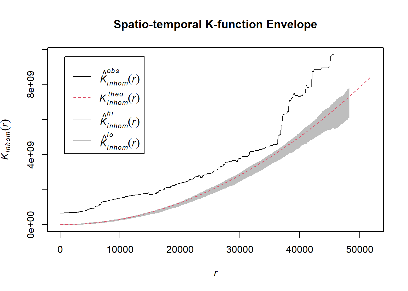
# Assuming `acled_spatio_ppp_owin` is your spatio-temporal point pattern object:
acled_spatio_ppp_owin <- magway_acled_quarters_2022_ppp[magway_owin]
K_st <- Kinhom(acled_spatio_ppp_owin, correction="border")
# Plot the result for visual inspection
plot(K_st, main = "Spatio-temporal K-function", legend=TRUE)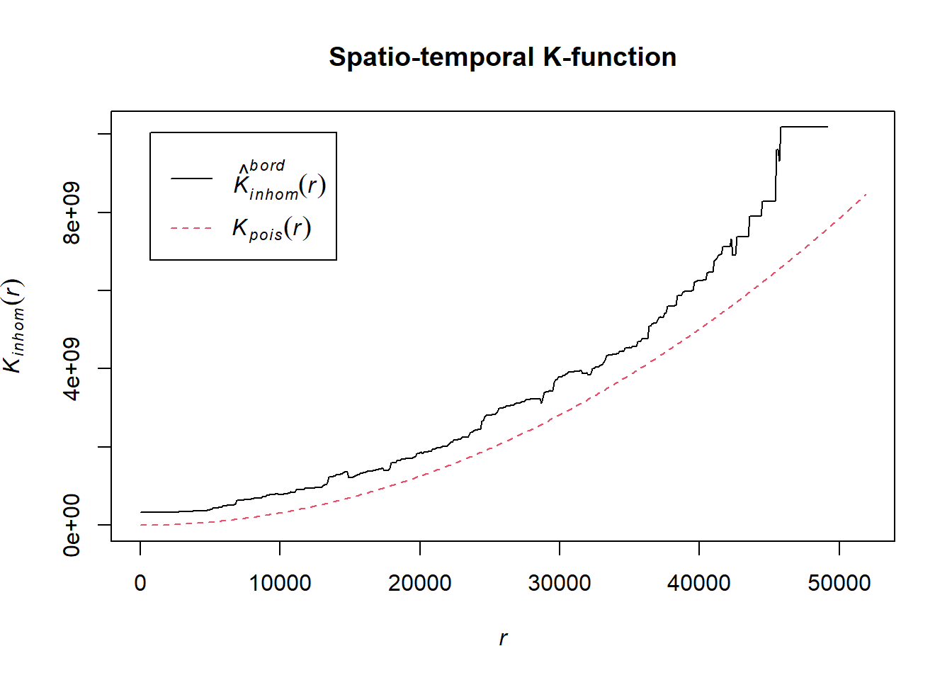
# Perform the CSR test with 99 simulations
K_ck.csr <- envelope(acled_spatio_ppp_owin, Kinhom, nsim=99, correction="border", parallel = parallel::detectCores())Generating 99 simulations of CSR ...
1, 2, 3, 4, 5, 6, 7, 8, 9, 10, 11, 12, 13, 14, 15, 16, 17, 18, 19, 20,
21, 22, 23, 24, 25, 26, 27, 28, 29, 30, 31, 32, 33, 34, 35, 36, 37, 38, 39, 40,
41, 42, 43, 44, 45, 46, 47, 48, 49, 50, 51, 52, 53, 54, 55, 56, 57, 58, 59, 60,
61, 62, 63, 64, 65, 66, 67, 68, 69, 70, 71, 72, 73, 74, 75, 76, 77, 78, 79, 80,
81, 82, 83, 84, 85, 86, 87, 88, 89, 90, 91, 92, 93, 94, 95, 96, 97, 98,
99.
Done.# Plot the envelope with the observed K-function
plot(K_ck.csr, main="Spatio-temporal K-function Envelope", legend=TRUE)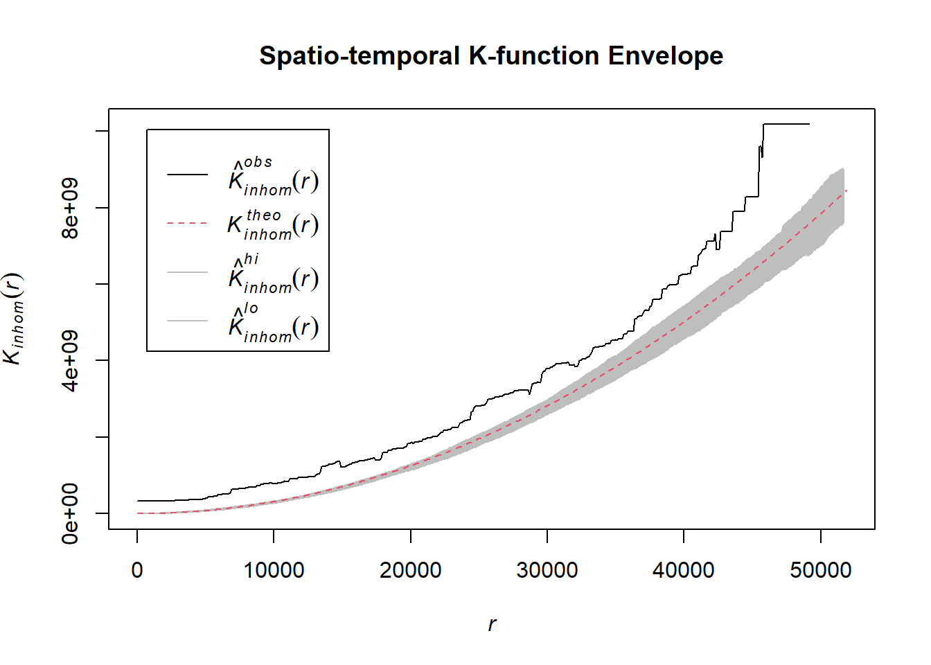
# Assuming `acled_spatio_ppp_owin` is your spatio-temporal point pattern object:
acled_spatio_ppp_owin <- magway_acled_quarters_2023_ppp[magway_owin]
K_st <- Kinhom(acled_spatio_ppp_owin, correction="border")
# Plot the result for visual inspection
plot(K_st, main = "Spatio-temporal K-function", legend=TRUE)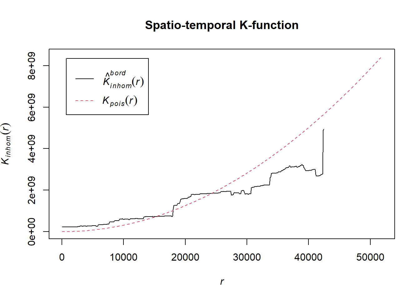
# Perform the CSR test with 99 simulations
K_ck.csr <- envelope(acled_spatio_ppp_owin, Kinhom, nsim=99, correction="border", parallel = parallel::detectCores())Generating 99 simulations of CSR ...
1, 2, 3, 4, 5, 6, 7, 8, 9, 10, 11, 12, 13, 14, 15, 16, 17, 18, 19, 20,
21, 22, 23, 24, 25, 26, 27, 28, 29, 30, 31, 32, 33, 34, 35, 36, 37, 38, 39, 40,
41, 42, 43, 44, 45, 46, 47, 48, 49, 50, 51, 52, 53, 54, 55, 56, 57, 58, 59, 60,
61, 62, 63, 64, 65, 66, 67, 68, 69, 70, 71, 72, 73, 74, 75, 76, 77, 78, 79, 80,
81, 82, 83, 84, 85, 86, 87, 88, 89, 90, 91, 92, 93, 94, 95, 96, 97, 98,
99.
Done.# Plot the envelope with the observed K-function
plot(K_ck.csr, main="Spatio-temporal K-function Envelope", legend=TRUE)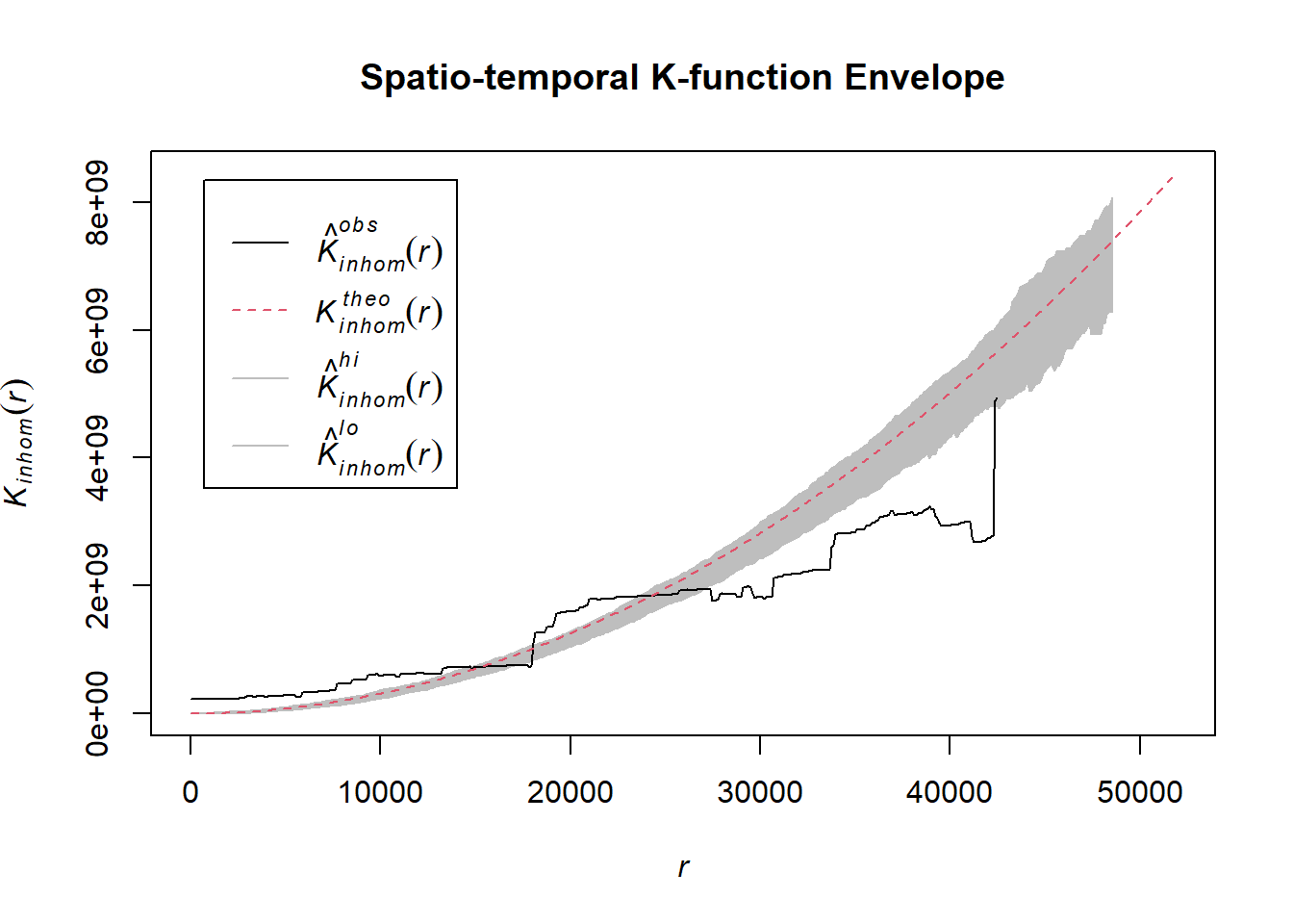
# Assuming `acled_spatio_ppp_owin` is your spatio-temporal point pattern object:
acled_spatio_ppp_owin <- magway_acled_quarters_2024_ppp[magway_owin]
K_st <- Kinhom(acled_spatio_ppp_owin, correction="border")
# Plot the result for visual inspection
plot(K_st, main = "Spatio-temporal K-function", legend=TRUE)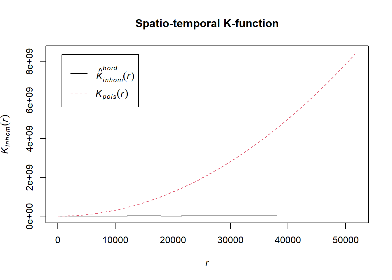
# Perform the CSR test with 99 simulations
K_ck.csr <- envelope(acled_spatio_ppp_owin, Kinhom, nsim=99, correction="border", parallel = parallel::detectCores())Generating 99 simulations of CSR ...
1, 2, 3, 4, 5, 6, 7, 8, 9, 10, 11, 12, 13, 14, 15, 16, 17, 18, 19, 20,
21, 22, 23, 24, 25, 26, 27, 28, 29, 30, 31, 32, 33, 34, 35, 36, 37, 38, 39, 40,
41, 42, 43, 44, 45, 46, 47, 48, 49, 50, 51, 52, 53, 54, 55, 56, 57, 58, 59, 60,
61, 62, 63, 64, 65, 66, 67, 68, 69, 70, 71, 72, 73, 74, 75, 76, 77, 78, 79, 80,
81, 82, 83, 84, 85, 86, 87, 88, 89, 90, 91, 92, 93, 94, 95, 96, 97, 98,
99.
Done.# Plot the envelope with the observed K-function
plot(K_ck.csr, main="Spatio-temporal K-function Envelope", legend=TRUE)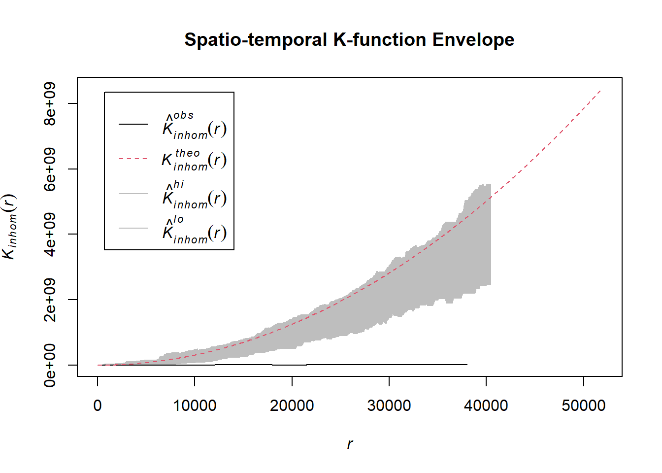
1.8.4.2.3 Battles
Example <- "Battles"
magway_acled_quarters_2021_ppp <- as.ppp(magway_acled_sf %>%
filter(year == 2021 & event_type == Example) %>%
select(q))
magway_acled_quarters_2022_ppp <- as.ppp(magway_acled_sf %>%
filter(year == 2022 & event_type == Example) %>%
select(q))
magway_acled_quarters_2023_ppp <- as.ppp(magway_acled_sf %>%
filter(year == 2023 & event_type == Example) %>%
select(q))
magway_acled_quarters_2024_ppp <- as.ppp(magway_acled_sf %>%
filter(year == 2024 & event_type == Example) %>%
select(q))# Assuming `acled_spatio_ppp_owin` is your spatio-temporal point pattern object:
acled_spatio_ppp_owin <- magway_acled_quarters_2021_ppp[magway_owin]
K_st <- Kinhom(acled_spatio_ppp_owin, correction="border")
# Plot the result for visual inspection
plot(K_st, main = "Spatio-temporal K-function", legend=TRUE)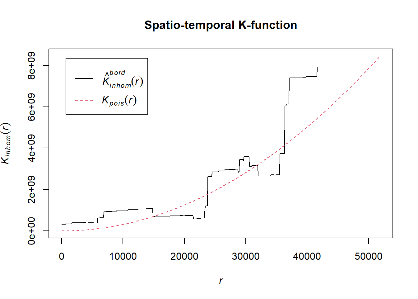
# Perform the CSR test with 99 simulations
K_ck.csr <- envelope(acled_spatio_ppp_owin, Kinhom, nsim=99, correction="border", parallel = parallel::detectCores())Generating 99 simulations of CSR ...
1, 2, 3, 4, 5, 6, 7, 8, 9, 10, 11, 12, 13, 14, 15, 16, 17, 18, 19, 20,
21, 22, 23, 24, 25, 26, 27, 28, 29, 30, 31, 32, 33, 34, 35, 36, 37, 38, 39, 40,
41, 42, 43, 44, 45, 46, 47, 48, 49, 50, 51, 52, 53, 54, 55, 56, 57, 58, 59, 60,
61, 62, 63, 64, 65, 66, 67, 68, 69, 70, 71, 72, 73, 74, 75, 76, 77, 78, 79, 80,
81, 82, 83, 84, 85, 86, 87, 88, 89, 90, 91, 92, 93, 94, 95, 96, 97, 98,
99.
Done.# Plot the envelope with the observed K-function
plot(K_ck.csr, main="Spatio-temporal K-function Envelope", legend=TRUE)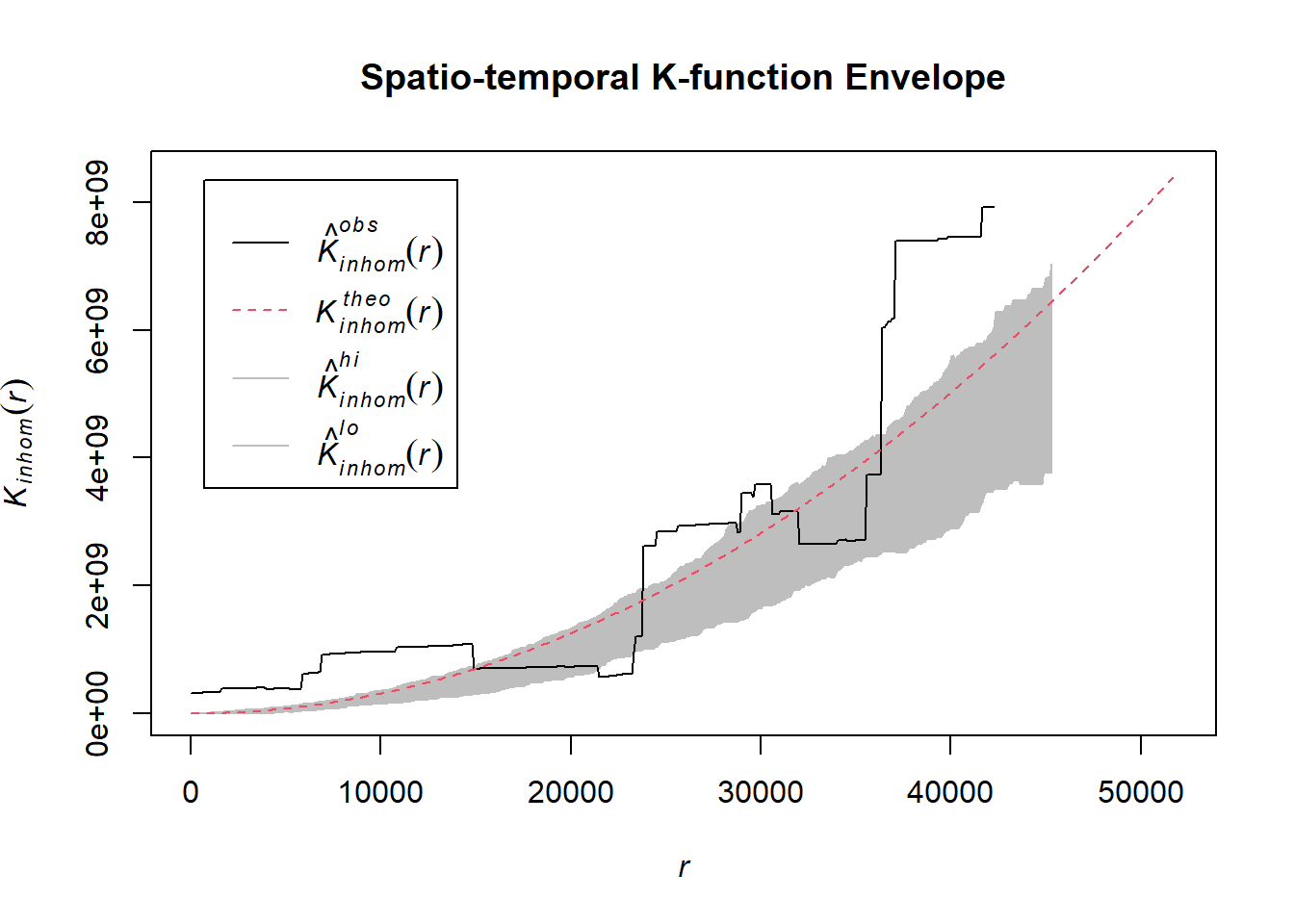
# Assuming `acled_spatio_ppp_owin` is your spatio-temporal point pattern object:
acled_spatio_ppp_owin <- magway_acled_quarters_2022_ppp[magway_owin]
K_st <- Kinhom(acled_spatio_ppp_owin, correction="border")
# Plot the result for visual inspection
plot(K_st, main = "Spatio-temporal K-function", legend=TRUE)
# Perform the CSR test with 99 simulations
K_ck.csr <- envelope(acled_spatio_ppp_owin, Kinhom, nsim=99, correction="border", parallel = parallel::detectCores())Generating 99 simulations of CSR ...
1, 2, 3, 4, 5, 6, 7, 8, 9, 10, 11, 12, 13, 14, 15, 16, 17, 18, 19, 20,
21, 22, 23, 24, 25, 26, 27, 28, 29, 30, 31, 32, 33, 34, 35, 36, 37, 38, 39, 40,
41, 42, 43, 44, 45, 46, 47, 48, 49, 50, 51, 52, 53, 54, 55, 56, 57, 58, 59, 60,
61, 62, 63, 64, 65, 66, 67, 68, 69, 70, 71, 72, 73, 74, 75, 76, 77, 78, 79, 80,
81, 82, 83, 84, 85, 86, 87, 88, 89, 90, 91, 92, 93, 94, 95, 96, 97, 98,
99.
Done.# Plot the envelope with the observed K-function
plot(K_ck.csr, main="Spatio-temporal K-function Envelope", legend=TRUE)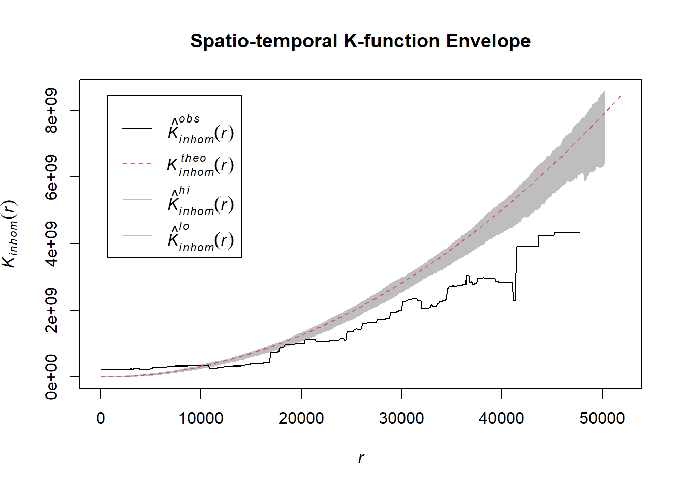
# Assuming `acled_spatio_ppp_owin` is your spatio-temporal point pattern object:
acled_spatio_ppp_owin <- magway_acled_quarters_2023_ppp[magway_owin]
K_st <- Kinhom(acled_spatio_ppp_owin, correction="border")
# Plot the result for visual inspection
plot(K_st, main = "Spatio-temporal K-function", legend=TRUE)
# Perform the CSR test with 99 simulations
K_ck.csr <- envelope(acled_spatio_ppp_owin, Kinhom, nsim=99, correction="border", parallel = parallel::detectCores())Generating 99 simulations of CSR ...
1, 2, 3, 4, 5, 6, 7, 8, 9, 10, 11, 12, 13, 14, 15, 16, 17, 18, 19, 20,
21, 22, 23, 24, 25, 26, 27, 28, 29, 30, 31, 32, 33, 34, 35, 36, 37, 38, 39, 40,
41, 42, 43, 44, 45, 46, 47, 48, 49, 50, 51, 52, 53, 54, 55, 56, 57, 58, 59, 60,
61, 62, 63, 64, 65, 66, 67, 68, 69, 70, 71, 72, 73, 74, 75, 76, 77, 78, 79, 80,
81, 82, 83, 84, 85, 86, 87, 88, 89, 90, 91, 92, 93, 94, 95, 96, 97, 98,
99.
Done.# Plot the envelope with the observed K-function
plot(K_ck.csr, main="Spatio-temporal K-function Envelope", legend=TRUE)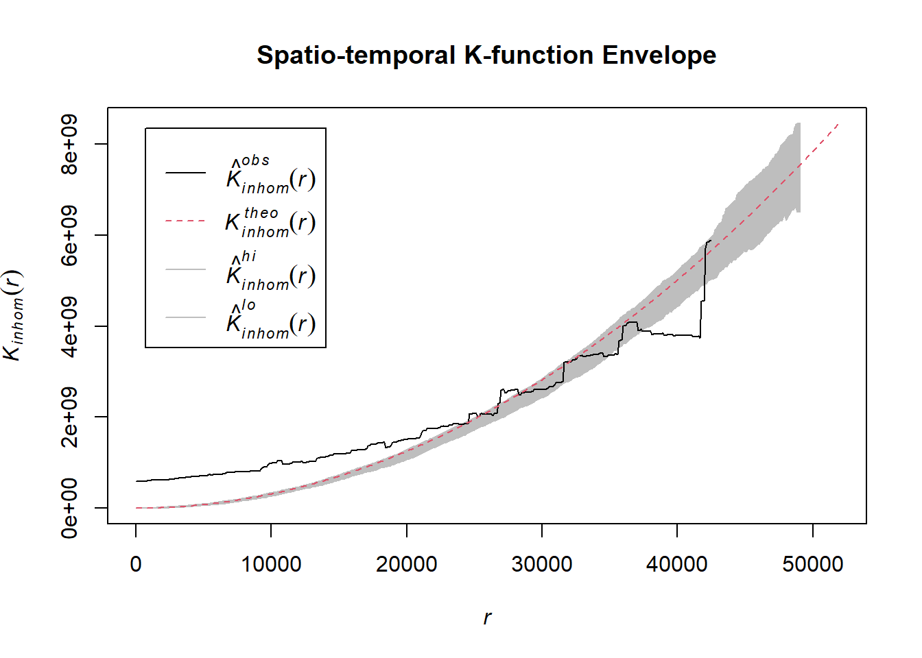
# Assuming `acled_spatio_ppp_owin` is your spatio-temporal point pattern object:
acled_spatio_ppp_owin <- magway_acled_quarters_2024_ppp[magway_owin]
K_st <- Kinhom(acled_spatio_ppp_owin, correction="border")
# Plot the result for visual inspection
plot(K_st, main = "Spatio-temporal K-function", legend=TRUE)
# Perform the CSR test with 99 simulations
K_ck.csr <- envelope(acled_spatio_ppp_owin, Kinhom, nsim=99, correction="border", parallel = parallel::detectCores())Generating 99 simulations of CSR ...
1, 2, 3, 4, 5, 6, 7, 8, 9, 10, 11, 12, 13, 14, 15, 16, 17, 18, 19, 20,
21, 22, 23, 24, 25, 26, 27, 28, 29, 30, 31, 32, 33, 34, 35, 36, 37, 38, 39, 40,
41, 42, 43, 44, 45, 46, 47, 48, 49, 50, 51, 52, 53, 54, 55, 56, 57, 58, 59, 60,
61, 62, 63, 64, 65, 66, 67, 68, 69, 70, 71, 72, 73, 74, 75, 76, 77, 78, 79, 80,
81, 82, 83, 84, 85, 86, 87, 88, 89, 90, 91, 92, 93, 94, 95, 96, 97, 98,
99.
Done.# Plot the envelope with the observed K-function
plot(K_ck.csr, main="Spatio-temporal K-function Envelope", legend=TRUE)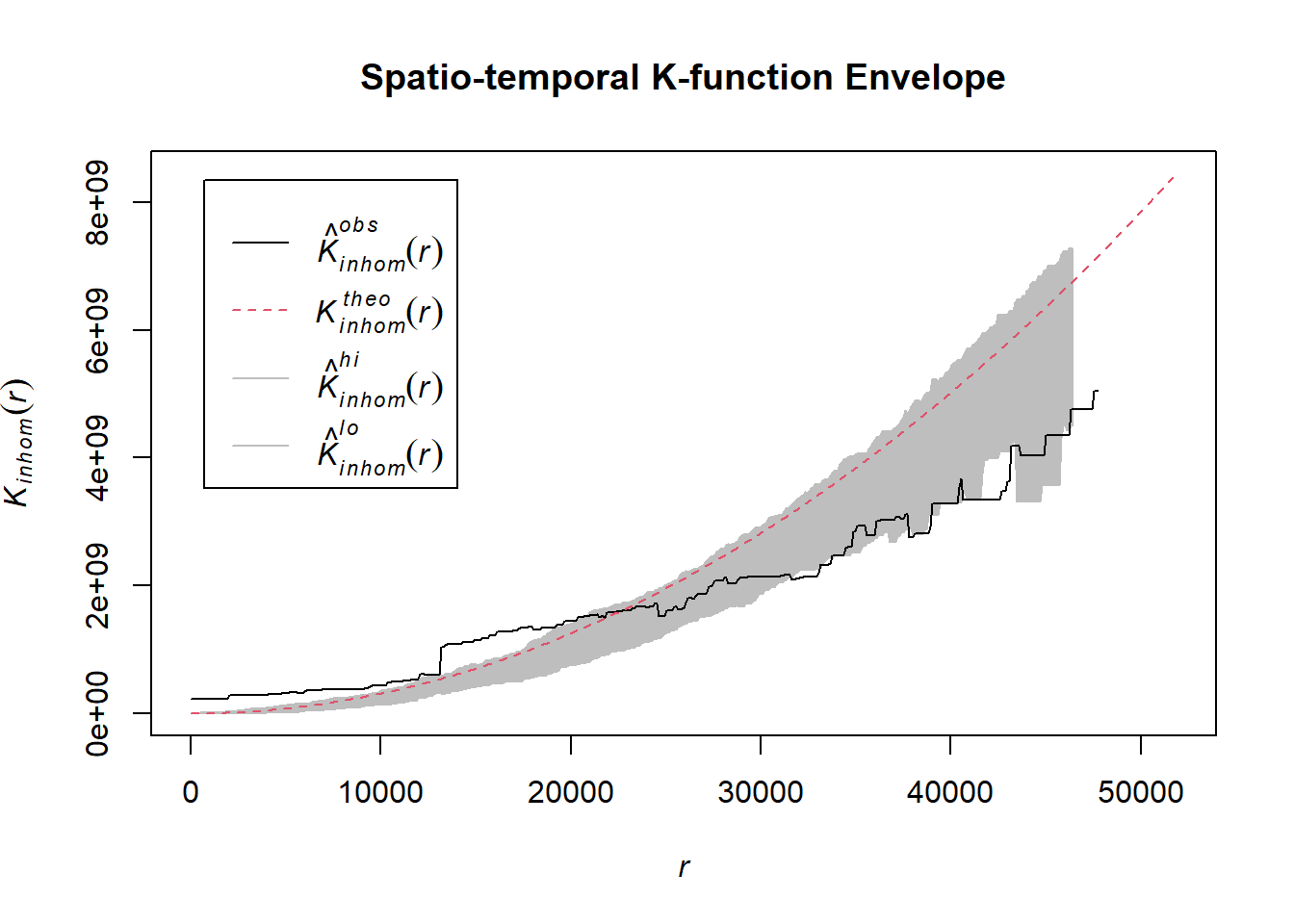
1.8.4.2.4 Violence against civilians
Example <- "Violence against civilians"
acled_quarters_2021_ppp <- as.ppp(temporal_acled_sf %>%
filter(year == 2021 & event_type == Example) %>%
select(q))
acled_quarters_2022_ppp <- as.ppp(temporal_acled_sf %>%
filter(year == 2022 & event_type == Example) %>%
select(q))
acled_quarters_2023_ppp <- as.ppp(temporal_acled_sf %>%
filter(year == 2023 & event_type == Example) %>%
select(q))
acled_quarters_2024_ppp <- as.ppp(temporal_acled_sf %>%
filter(year == 2024 & event_type == Example) %>%
select(q))# Assuming `acled_spatio_ppp_owin` is your spatio-temporal point pattern object:
acled_spatio_ppp_owin <- magway_acled_quarters_2021_ppp[magway_owin]
K_st <- Kinhom(acled_spatio_ppp_owin, correction="border")
# Plot the result for visual inspection
plot(K_st, main = "Spatio-temporal K-function", legend=TRUE)
# Perform the CSR test with 99 simulations
K_ck.csr <- envelope(acled_spatio_ppp_owin, Kinhom, nsim=99, correction="border", parallel = parallel::detectCores())Generating 99 simulations of CSR ...
1, 2, 3, 4, 5, 6, 7, 8, 9, 10, 11, 12, 13, 14, 15, 16, 17, 18, 19, 20,
21, 22, 23, 24, 25, 26, 27, 28, 29, 30, 31, 32, 33, 34, 35, 36, 37, 38, 39, 40,
41, 42, 43, 44, 45, 46, 47, 48, 49, 50, 51, 52, 53, 54, 55, 56, 57, 58, 59, 60,
61, 62, 63, 64, 65, 66, 67, 68, 69, 70, 71, 72, 73, 74, 75, 76, 77, 78, 79, 80,
81, 82, 83, 84, 85, 86, 87, 88, 89, 90, 91, 92, 93, 94, 95, 96, 97, 98,
99.
Done.# Plot the envelope with the observed K-function
plot(K_ck.csr, main="Spatio-temporal K-function Envelope", legend=TRUE)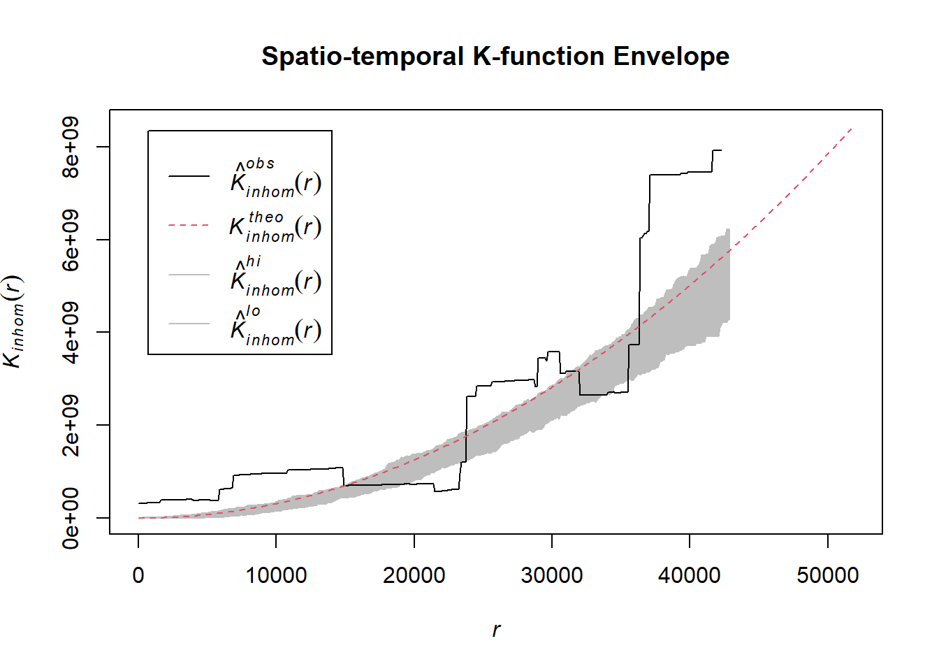
# Assuming `acled_spatio_ppp_owin` is your spatio-temporal point pattern object:
acled_spatio_ppp_owin <- magway_acled_quarters_2022_ppp[magway_owin]
K_st <- Kinhom(acled_spatio_ppp_owin, correction="border")
# Plot the result for visual inspection
plot(K_st, main = "Spatio-temporal K-function", legend=TRUE)
# Perform the CSR test with 99 simulations
K_ck.csr <- envelope(acled_spatio_ppp_owin, Kinhom, nsim=99, correction="border", parallel = parallel::detectCores())Generating 99 simulations of CSR ...
1, 2, 3, 4, 5, 6, 7, 8, 9, 10, 11, 12, 13, 14, 15, 16, 17, 18, 19, 20,
21, 22, 23, 24, 25, 26, 27, 28, 29, 30, 31, 32, 33, 34, 35, 36, 37, 38, 39, 40,
41, 42, 43, 44, 45, 46, 47, 48, 49, 50, 51, 52, 53, 54, 55, 56, 57, 58, 59, 60,
61, 62, 63, 64, 65, 66, 67, 68, 69, 70, 71, 72, 73, 74, 75, 76, 77, 78, 79, 80,
81, 82, 83, 84, 85, 86, 87, 88, 89, 90, 91, 92, 93, 94, 95, 96, 97, 98,
99.
Done.# Plot the envelope with the observed K-function
plot(K_ck.csr, main="Spatio-temporal K-function Envelope", legend=TRUE)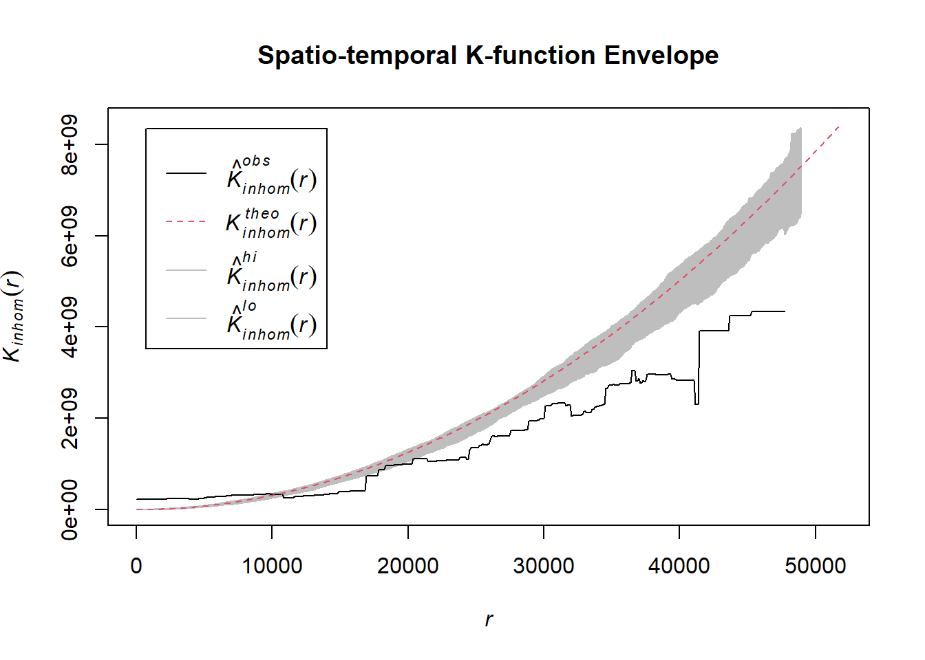
# Assuming `acled_spatio_ppp_owin` is your spatio-temporal point pattern object:
acled_spatio_ppp_owin <- magway_acled_quarters_2023_ppp[magway_owin]
K_st <- Kinhom(acled_spatio_ppp_owin, correction="border")
# Plot the result for visual inspection
plot(K_st, main = "Spatio-temporal K-function", legend=TRUE)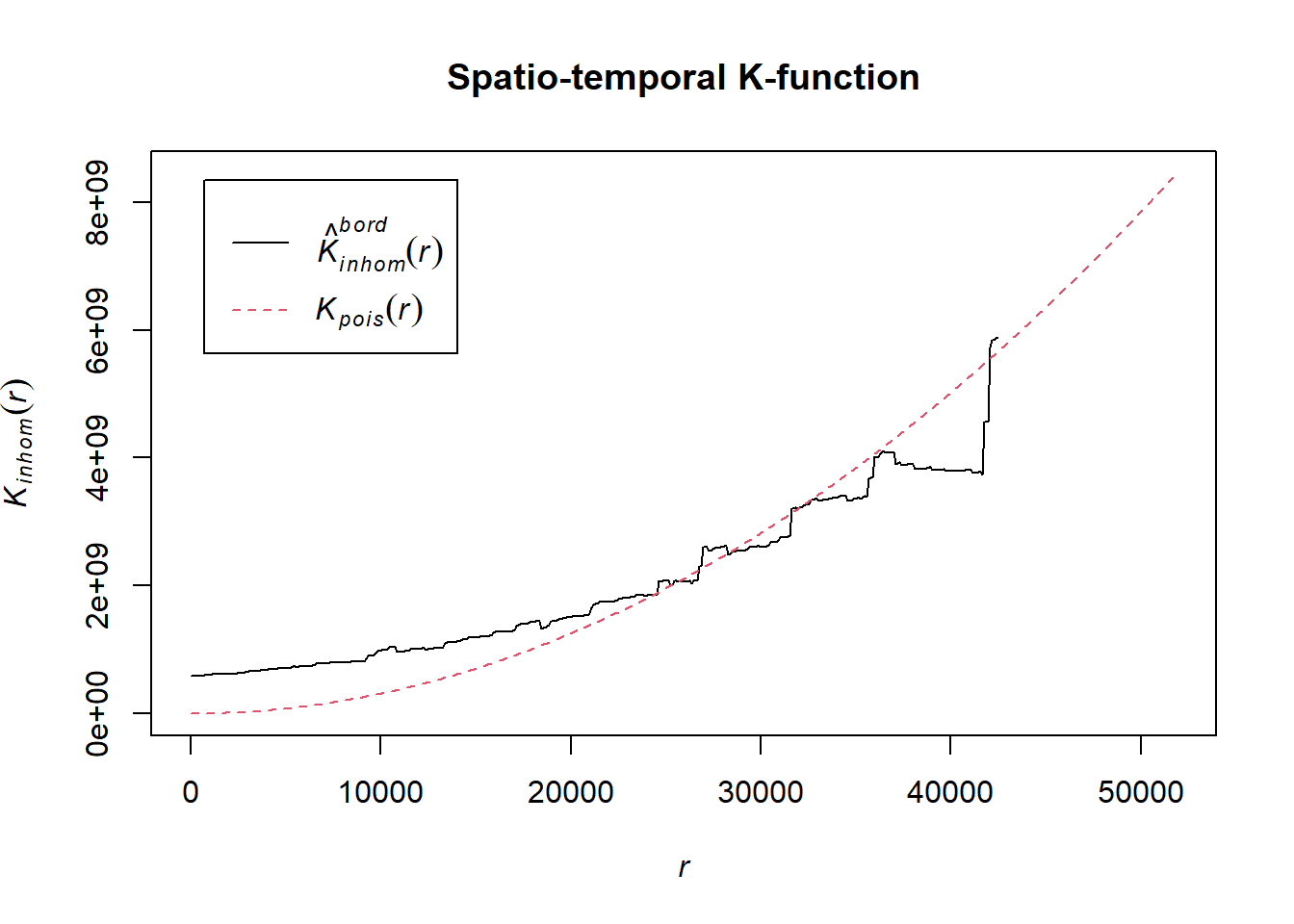
# Perform the CSR test with 99 simulations
K_ck.csr <- envelope(acled_spatio_ppp_owin, Kinhom, nsim=99, correction="border", parallel = parallel::detectCores())Generating 99 simulations of CSR ...
1, 2, 3, 4, 5, 6, 7, 8, 9, 10, 11, 12, 13, 14, 15, 16, 17, 18, 19, 20,
21, 22, 23, 24, 25, 26, 27, 28, 29, 30, 31, 32, 33, 34, 35, 36, 37, 38, 39, 40,
41, 42, 43, 44, 45, 46, 47, 48, 49, 50, 51, 52, 53, 54, 55, 56, 57, 58, 59, 60,
61, 62, 63, 64, 65, 66, 67, 68, 69, 70, 71, 72, 73, 74, 75, 76, 77, 78, 79, 80,
81, 82, 83, 84, 85, 86, 87, 88, 89, 90, 91, 92, 93, 94, 95, 96, 97, 98,
99.
Done.# Plot the envelope with the observed K-function
plot(K_ck.csr, main="Spatio-temporal K-function Envelope", legend=TRUE)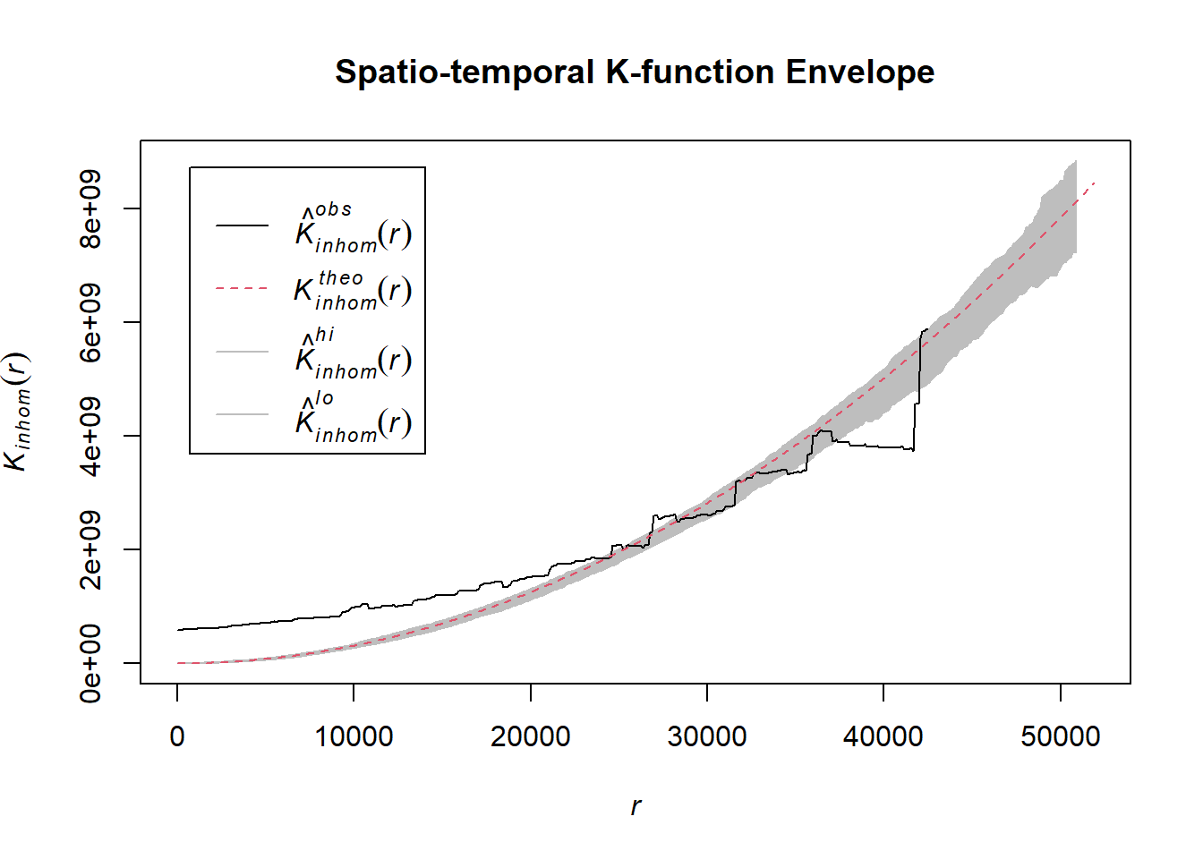
# Assuming `acled_spatio_ppp_owin` is your spatio-temporal point pattern object:
acled_spatio_ppp_owin <- magway_acled_quarters_2024_ppp[magway_owin]
K_st <- Kinhom(acled_spatio_ppp_owin, correction="border")
# Plot the result for visual inspection
plot(K_st, main = "Spatio-temporal K-function", legend=TRUE)
# Perform the CSR test with 99 simulations
K_ck.csr <- envelope(acled_spatio_ppp_owin, Kinhom, nsim=99, correction="border", parallel = parallel::detectCores())Generating 99 simulations of CSR ...
1, 2, 3, 4, 5, 6, 7, 8, 9, 10, 11, 12, 13, 14, 15, 16, 17, 18, 19, 20,
21, 22, 23, 24, 25, 26, 27, 28, 29, 30, 31, 32, 33, 34, 35, 36, 37, 38, 39, 40,
41, 42, 43, 44, 45, 46, 47, 48, 49, 50, 51, 52, 53, 54, 55, 56, 57, 58, 59, 60,
61, 62, 63, 64, 65, 66, 67, 68, 69, 70, 71, 72, 73, 74, 75, 76, 77, 78, 79, 80,
81, 82, 83, 84, 85, 86, 87, 88, 89, 90, 91, 92, 93, 94, 95, 96, 97, 98,
99.
Done.# Plot the envelope with the observed K-function
plot(K_ck.csr, main="Spatio-temporal K-function Envelope", legend=TRUE)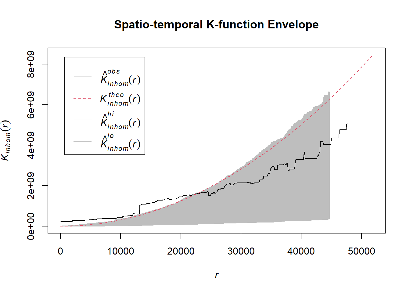
Note
Interpretation:
In general, the observed K-function (black line) starts within the envelope but begins to deviate upward as the spatial distance increases, crossing beyond the envelope at larger distances.
This suggests that possible **spatio-temporal clustering) is occurring at larger distances beyond the theoretical expectations under complete randomness.
The envelope allows for a statistical comparison: if the observed K-function exceeds the envelope, it implies significant clustering at those distances.
This plot suggests that the observed pattern of events is not completely random and that significant clustering occurs at larger spatial distances and time intervals, which can reveal important insights about the underlying structure of the event occurrences.
Thus, these clusterings could suggests the following:
- Non-Random Targeting and Temporal Patterns:
- The non-random nature of the observed patterns implies that conflict actors may be targeting specific regions repeatedly over certain periods, driven by strategic or political goals.
- This could point to strategically significant areas like important roads, military installations, or regions with ethnic minorities being hotspots of repeated violence.
- Localized Hotspots of Conflict:
- The clustering pattern at larger distances implies that violent events, such as battles or civilian attacks, are concentrated in certain regions rather than being evenly spread across the country.
- Regions like Chin, Sagaing, Magway, and Mandalay, which have been reported as key areas of conflict, experience recurring waves of violence concentrated in specific localities, due strategic importance, military operations, or political importance.
1.9 Conclusion
The war in Myanmar has involved numerous armed groups, including pro-democracy forces and ethnic militias, battling against the military junta. The situation remains highly volatile, with frequent battles occurring across various regions, including Chin, Sagaing, Magway, and Mandalay. The conflict exhibits a cyclical nature, with periods of relative calm punctuated by intense fighting, particularly during dry seasons.
Myanmar’s political future remains uncertain, with the ongoing struggle between resistance forces and the military junta casting doubt over the country’s ability to maintain unity and stability.
References - BBC News. (2021). ‘Mandalay was a massacre’: Security forces fire at protests. Retrieved from https://www.bbc.com/news/world-asia-56386348
Thit, N. (2022). How Sagaing Is at Forefront of Revolution Against Myanmar’s Junta. Retrieved from https://www.irrawaddy.com/opinion/analysis/how-sagaing-is-at-forefront-of-revolution-against-myanmars-junta.html
ND-Burma (2024). Human Rights Violations took place in States and Regions from Aug 22 to 31, 2024. Retrieved from https://reliefweb.int/report/myanmar/human-rights-situation-weekly-update-aug-22-31-2024-enmy
ND-Burma (2024). Human Rights Violations took place in States and Regions from Aug 15 to 21, 2024. Retrieved from https://reliefweb.int/report/myanmar/human-rights-situation-weekly-update-aug-15-21-2024-enmy
ND-Burma (2024). Human Rights Violations took place in States and Regions from Sep 1 to 7, 2024. Retrieved from https://reliefweb.int/report/myanmar/human-rights-situation-weekly-update-september-1-7-2024-enmy