pacman::p_load(sf, spdep, tmap, tidyverse, knitr, GWmodel)In Class exercise 5
Analysis
R
sf
tidyverse
5.0 Notes:
A way to define spatial neighbourhood (Polygon vs Centroid)
Defining spatial weights
Using a centroid to determine the neighhours around a particular area
centroid would be able to gauge how far any neighbour is close to the area in focus
- Limitations of centroid: irregular shaped areas, land
Contiguity Neighbours
Common shared boundary
- Rook’s case, Bishop’s case, Queen’s case
Multiple order used in measuring contiguity
Can be seen a graph with differing cases focusing on where their neighbours are connected
5.1 Installing and Loading the R packages
For the purpose of this study, five R packages will be used. They are:
sf, a relatively new R package specially designed to import, manage and process vector-based geospatial data in R.
spatstat, a comprehensive package for point pattern analysis. We’ll use it to perform first- and second-order spatial point pattern analyses and to derive kernel density estimation (KDE) layers.
spdep, an R package focused on spatial dependence and spatial econometrics. It includes functions for computing spatial weights, neighborhood structures, and spatially lagged variables, which are crucial for understanding spatial relationships in data.
knitr, an R package that enables dynamic report generation. It integrates R code with Markdown or LaTeX to create reproducible documents, which is useful for documenting and sharing your analysis workflows.
tidyverse, a collection of R packages designed for data science. It includes packages like
dplyrfor data manipulation,ggplot2for data visualization, andtidyrfor data tidying, all of which are essential for handling and analyzing data efficiently in a clean and consistent manner.GWmodel, a collection of techniques from a particular branch of spatial statistics,termed geographically-weighted (GW) models. GW models suit situations when data are not described well by some global model, but where there are spatial regions where a suitably localised calibration provides a better description.
5.1.1 Import shapefile into r environment
The code chunk below uses st_read() of sf package to import Hunan shapefile into R. The imported shapefile will be simple features Object of sf.
hunan_sf <- st_read(dsn = "data/In-class_Ex05/geospatial",
                 layer = "Hunan")
Reading layer `Hunan' from data source
`C:\Users\blzll\OneDrive\Desktop\Y3S1\IS415\Quarto\IS415\In-class_Ex\data\In-class_Ex05\geospatial'
using driver `ESRI Shapefile'
Simple feature collection with 88 features and 7 fields
Geometry type: POLYGON
Dimension: XY
Bounding box: xmin: 108.7831 ymin: 24.6342 xmax: 114.2544 ymax: 30.12812
Geodetic CRS: WGS 845.1.2 Import csv file into r environment
Next, we will import Hunan_2012.csv into R by using read_csv() of readr package. The output is R dataframe class.
hunan2012 <- read_csv("data/In-class_Ex05/aspatial/Hunan_2012.csv")
hunan2012
# A tibble: 88 × 29
County City avg_wage deposite FAI Gov_Rev Gov_Exp GDP GDPPC GIO
<chr> <chr> <dbl> <dbl> <dbl> <dbl> <dbl> <dbl> <dbl> <dbl>
1 Anhua Yiyang 30544 10967 6832. 457. 2703 13225 14567 9277.
2 Anren Chenz… 28058 4599. 6386. 221. 1455. 4941. 12761 4189.
3 Anxiang Chang… 31935 5517. 3541 244. 1780. 12482 23667 5109.
4 Baojing Hunan… 30843 2250 1005. 193. 1379. 4088. 14563 3624.
5 Chaling Zhuzh… 31251 8241. 6508. 620. 1947 11585 20078 9158.
6 Changning Hengy… 28518 10860 7920 770. 2632. 19886 24418 37392
7 Changsha Chang… 54540 24332 33624 5350 7886. 88009 88656 51361
8 Chengbu Shaoy… 28597 2581. 1922. 161. 1192. 2570. 10132 1681.
9 Chenxi Huaih… 33580 4990 5818. 460. 1724. 7755. 17026 6644.
10 Cili Zhang… 33099 8117. 4498. 500. 2306. 11378 18714 5843.
# ℹ 78 more rows
# ℹ 19 more variables: Loan <dbl>, NIPCR <dbl>, Bed <dbl>, Emp <dbl>,
# EmpR <dbl>, EmpRT <dbl>, Pri_Stu <dbl>, Sec_Stu <dbl>, Household <dbl>,
# Household_R <dbl>, NOIP <dbl>, Pop_R <dbl>, RSCG <dbl>, Pop_T <dbl>,
# Agri <dbl>, Service <dbl>, Disp_Inc <dbl>, RORP <dbl>, ROREmp <dbl>5.1.3 Performing relational join
The code chunk below will be used to update the attribute table of hunan’s SpatialPolygonsDataFrame with the attribute fields of hunan2012 data frame. This is performed by using left_join() of dplyr package.
hunan_sf <- left_join(hunan_sf,hunan2012)%>%
  select(1:3, 7, 15, 16, 31, 32)
5.1.4 Store file locally
Writing to rds would allow for quick retrieval of required data
hunan_sf <- read_rds("data/rds/hunan_sf.rds")5.2 Converting to SpatialPolgyonDataFrame
hunan_sp <- hunan_sf %>%
  as_Spatial()
5.3 Geographically Weighted Summary Statistics with Adaptive Bandwidth
Akaike information criterion (AIC) approach to determine the recommended number of neighbours
bw_AIC_adapt <- bw.gwr(GDPPC ~ 1,
                 data = hunan_sp,
                 approach = 'AIC',
                 adaptive = TRUE,
                 kernel = 'bisquare',
                 longlat = T)
Adaptive bandwidth (number of nearest neighbours): 62 AICc value: 1923.156
Adaptive bandwidth (number of nearest neighbours): 46 AICc value: 1920.469
Adaptive bandwidth (number of nearest neighbours): 36 AICc value: 1917.324
Adaptive bandwidth (number of nearest neighbours): 29 AICc value: 1916.661
Adaptive bandwidth (number of nearest neighbours): 26 AICc value: 1914.897
Adaptive bandwidth (number of nearest neighbours): 22 AICc value: 1914.045
Adaptive bandwidth (number of nearest neighbours): 22 AICc value: 1914.045 Cross validation approach to determine the recommended number of neighbours
bw_CV_adapt <- bw.gwr(GDPPC ~ 1,
                 data = hunan_sp,
                 approach = 'CV',
                 adaptive = TRUE,
                 kernel = 'bisquare',
                 longlat = T)
Adaptive bandwidth: 62 CV score: 15515442343
Adaptive bandwidth: 46 CV score: 14937956887
Adaptive bandwidth: 36 CV score: 14408561608
Adaptive bandwidth: 29 CV score: 14198527496
Adaptive bandwidth: 26 CV score: 13898800611
Adaptive bandwidth: 22 CV score: 13662299974
Adaptive bandwidth: 22 CV score: 13662299974 5.4 Geographically Weighted Summary Statistics with Fixed Bandwidth
Akaike information criterion (AIC) approach to determine the recommended number of neighbours
bw_AIC_fixed <- bw.gwr(GDPPC ~ 1,
                 data = hunan_sp,
                 approach = 'AIC',
                 adaptive = FALSE,
                 kernel = 'bisquare',
                 longlat = T)
Fixed bandwidth: 357.4897 AICc value: 1927.631
Fixed bandwidth: 220.985 AICc value: 1921.547
Fixed bandwidth: 136.6204 AICc value: 1919.993
Fixed bandwidth: 84.48025 AICc value: 1940.603
Fixed bandwidth: 168.8448 AICc value: 1919.457
Fixed bandwidth: 188.7606 AICc value: 1920.007
Fixed bandwidth: 156.5362 AICc value: 1919.41
Fixed bandwidth: 148.929 AICc value: 1919.527
Fixed bandwidth: 161.2377 AICc value: 1919.392
Fixed bandwidth: 164.1433 AICc value: 1919.403
Fixed bandwidth: 159.4419 AICc value: 1919.393
Fixed bandwidth: 162.3475 AICc value: 1919.394
Fixed bandwidth: 160.5517 AICc value: 1919.391 Cross validation approach to determine the recommended number of neighbours
bw_CV_fixed <- bw.gwr(GDPPC ~ 1,
                 data = hunan_sp,
                 approach = 'CV',
                 adaptive = FALSE,
                 kernel = 'bisquare',
                 longlat = T)
Fixed bandwidth: 357.4897 CV score: 16265191728
Fixed bandwidth: 220.985 CV score: 14954930931
Fixed bandwidth: 136.6204 CV score: 14134185837
Fixed bandwidth: 84.48025 CV score: 13693362460
Fixed bandwidth: 52.25585 CV score: Inf
Fixed bandwidth: 104.396 CV score: 13891052305
Fixed bandwidth: 72.17162 CV score: 13577893677
Fixed bandwidth: 64.56447 CV score: 14681160609
Fixed bandwidth: 76.8731 CV score: 13444716890
Fixed bandwidth: 79.77877 CV score: 13503296834
Fixed bandwidth: 75.07729 CV score: 13452450771
Fixed bandwidth: 77.98296 CV score: 13457916138
Fixed bandwidth: 76.18716 CV score: 13442911302
Fixed bandwidth: 75.76323 CV score: 13444600639
Fixed bandwidth: 76.44916 CV score: 13442994078
Fixed bandwidth: 76.02523 CV score: 13443285248
Fixed bandwidth: 76.28724 CV score: 13442844774
Fixed bandwidth: 76.34909 CV score: 13442864995
Fixed bandwidth: 76.24901 CV score: 13442855596
Fixed bandwidth: 76.31086 CV score: 13442847019
Fixed bandwidth: 76.27264 CV score: 13442846793
Fixed bandwidth: 76.29626 CV score: 13442844829
Fixed bandwidth: 76.28166 CV score: 13442845238
Fixed bandwidth: 76.29068 CV score: 13442844678
Fixed bandwidth: 76.29281 CV score: 13442844691
Fixed bandwidth: 76.28937 CV score: 13442844698
Fixed bandwidth: 76.2915 CV score: 13442844676
Fixed bandwidth: 76.292 CV score: 13442844679
Fixed bandwidth: 76.29119 CV score: 13442844676
Fixed bandwidth: 76.29099 CV score: 13442844676
Fixed bandwidth: 76.29131 CV score: 13442844676
Fixed bandwidth: 76.29138 CV score: 13442844676
Fixed bandwidth: 76.29126 CV score: 13442844676
Fixed bandwidth: 76.29123 CV score: 13442844676 It can be observed that unlike the determination of the adaptive bandwidth, fixed bandwidth yield vastly different results for the methods of AIC and Cross Validation
5.4 Geographically Weighted Summary Statistics with adaptive Bandwidth
gwstat <- gwss(data = hunan_sp,
               vars = "GDPPC",
               bw = bw_AIC_adapt,
               kernel = "bisquare",
               adaptive = TRUE,
               longlat = T)
gwstat[["SDF"]]
class : SpatialPolygonsDataFrame
features : 88
extent : 108.7831, 114.2544, 24.6342, 30.12812 (xmin, xmax, ymin, ymax)
crs : +proj=longlat +datum=WGS84 +no_defs
variables : 5
names : GDPPC_LM, GDPPC_LSD, GDPPC_LVar, GDPPC_LSKe, GDPPC_LCV
min values : 13688.6986033259, 4282.59917616925, 18340655.7037255, -0.215059890053628, 0.200050258645349
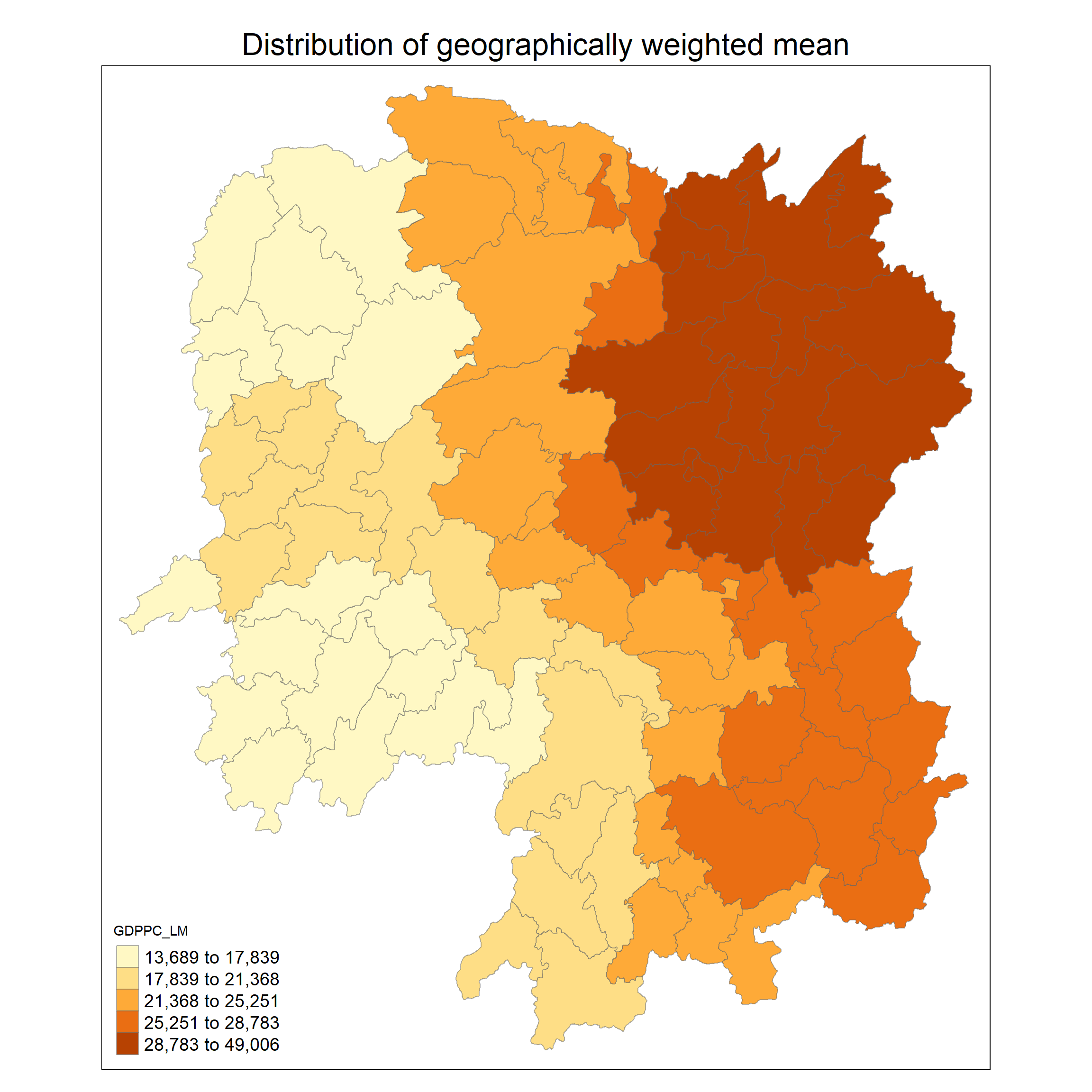
max values : 49005.8382943034, 22568.8411539952, 509352591.034267, 3.7525953469342, 0.801815253056721 Code chunk below is used to extract SDF data table from gwss object output from gwss(). It will be converted into data.frame by using as.data.frame()
gwstat_df <- as.data.frame(gwstat$SDF)Next, cbind() is used to append the newly derived data.frame onto hunan_sf sf data.frame in the code chunk below
hunan_gstat <- cbind(hunan_sf, gwstat_df)tm_shape(hunan_gstat) +
tm_fill("GDPPC_LM",
n = 5,
style = "quantile") +
tm_borders(alpha = 0.5) +
tm_layout(main.title = "Distribution of geographically weighted mean",
main.title.position = "center",
main.title.size = 2.0,
legend.text.size = 1.2,
legend.height = 1.50,
legend.width = 1.50,
frame = TRUE)