pacman::p_load(sf, spdep, GWmodel, SpatialML,
               tmap, rsample, yardstick, tidyverse,
knitr, kableExtra, spatialRF)In Class exercise 13
Analysis
R
sf
spdep
GWmodel
SpatialML
tmap
rsample
yardstick
tidyverse
knitr
kableExtra
spatialRF
Getting Started
Import the packages
Preparing Data
mdata <- read_rds("data/In-class_Ex13/rds/mdata.rds")Data Sampling
Calibrating predictive models are computational intensive, especially random forest method is used. For quick prototyping, a 10% sample will be selected at random from the data by using the code chunk below.
set.seed(1234)
HDB_sample <- mdata %>%
  sample_n(1500)
Checking of overlapping point
overlapping_points <- HDB_sample %>%
  mutate(overlap = lengths(st_equals(., .)) >1)
summary(overlapping_points$overlap)
Mode FALSE TRUE
logical 1047 453 Spatial jitter
HDB_sample <- HDB_sample %>%
  st_jitter(amount = 5)
Data Sampling for training/test data
set.seed(1234)
resale_split <- initial_split(HDB_sample,
                              prop = 6.67/10,)
train_data <- training(resale_split)
test_data <- testing(resale_split)write_rds(train_data, "data/In-class_Ex13/rds/train_data.rds")
write_rds(test_data, "data/In-class_Ex13/rds/test_data.rds")train_data <- read_rds("data/In-class_Ex13/rds/train_data.rds")
test_data <- read_rds("data/In-class_Ex13/rds/test_data.rds")Multicollinearity check
mdata_nogeo <- mdata %>%
  st_drop_geometry()
ggstatsplot::ggcorrmat(mdata_nogeo[,2:17], matrix.type = "full")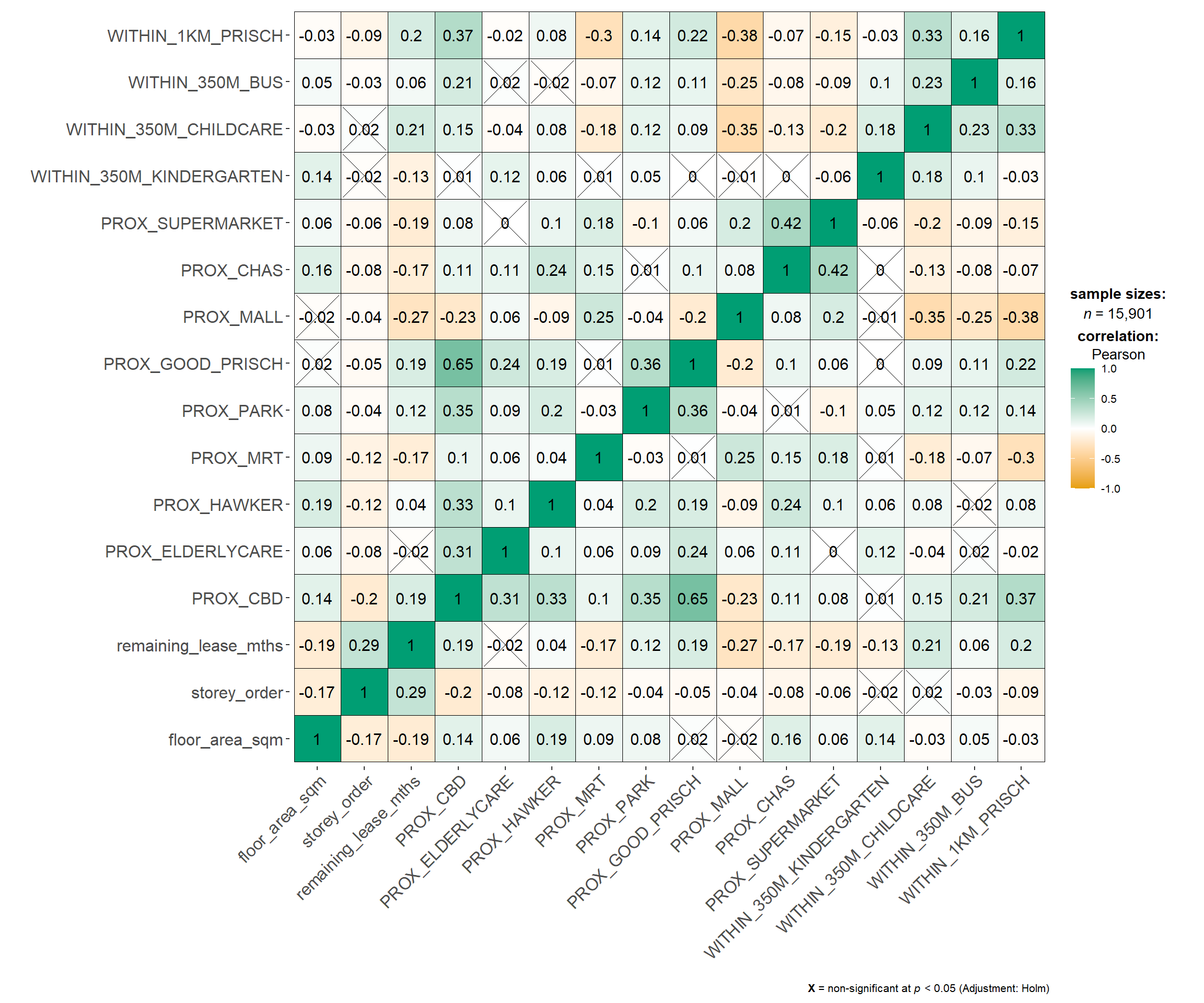
Building a non-spatial multiple linear regression
price_mlr <- lm(resale_price ~ floor_area_sqm +
                  storey_order + remaining_lease_mths +
                  PROX_CBD + PROX_ELDERLYCARE + PROX_HAWKER +
                  PROX_MRT + PROX_PARK + PROX_MALL +
                  PROX_SUPERMARKET + WITHIN_350M_KINDERGARTEN +
                  WITHIN_350M_CHILDCARE + WITHIN_350M_BUS +
                  WITHIN_1KM_PRISCH,
                data=train_data)
summary(price_mlr)
Call:
lm(formula = resale_price ~ floor_area_sqm + storey_order + remaining_lease_mths +
    PROX_CBD + PROX_ELDERLYCARE + PROX_HAWKER + PROX_MRT + PROX_PARK +
    PROX_MALL + PROX_SUPERMARKET + WITHIN_350M_KINDERGARTEN +
    WITHIN_350M_CHILDCARE + WITHIN_350M_BUS + WITHIN_1KM_PRISCH,
    data = train_data)

Residuals:
    Min      1Q  Median      3Q     Max
-205193  -39120   -1930   36545  472355

Coefficients:
                           Estimate Std. Error t value Pr(>|t|)
(Intercept)              107601.073  10601.261  10.150  < 2e-16 ***
floor_area_sqm             2780.698     90.579  30.699  < 2e-16 ***
storey_order              14299.298    339.115  42.167  < 2e-16 ***
remaining_lease_mths        344.490      4.592  75.027  < 2e-16 ***
PROX_CBD                 -16930.196    201.254 -84.124  < 2e-16 ***
PROX_ELDERLYCARE         -14441.025    994.867 -14.516  < 2e-16 ***
PROX_HAWKER              -19265.648   1273.597 -15.127  < 2e-16 ***
PROX_MRT                 -32564.272   1744.232 -18.670  < 2e-16 ***
PROX_PARK                 -5712.625   1483.885  -3.850 0.000119 ***
PROX_MALL                -14717.388   2007.818  -7.330 2.47e-13 ***
PROX_SUPERMARKET         -26881.938   4189.624  -6.416 1.46e-10 ***
WITHIN_350M_KINDERGARTEN   8520.472    632.812  13.464  < 2e-16 ***
WITHIN_350M_CHILDCARE     -4510.650    354.015 -12.741  < 2e-16 ***
WITHIN_350M_BUS             813.493    222.574   3.655 0.000259 ***
WITHIN_1KM_PRISCH         -8010.834    491.512 -16.298  < 2e-16 ***
---
Signif. codes:  0 '***' 0.001 '**' 0.01 '*' 0.05 '.' 0.1 ' ' 1

Residual standard error: 61650 on 10320 degrees of freedom
Multiple R-squared:  0.7373,    Adjusted R-squared:  0.737
F-statistic:  2069 on 14 and 10320 DF,  p-value: < 2.2e-16
Predictive Modelling with gwr
Computing bw
gwr_bw_train_ad <- bw.gwr(resale_price ~ floor_area_sqm +
                  storey_order + remaining_lease_mths +
                  PROX_CBD + PROX_ELDERLYCARE + PROX_HAWKER +
                  PROX_MRT + PROX_PARK + PROX_MALL +
                  PROX_SUPERMARKET + WITHIN_350M_KINDERGARTEN +
                  WITHIN_350M_CHILDCARE + WITHIN_350M_BUS +
                  WITHIN_1KM_PRISCH,
                  data=train_data,
                  approach="CV",
                  kernel="gaussian",
                  adaptive=TRUE,
                  longlat=FALSE)
Take a cup of tea and have a break, it will take a few minutes.
-----A kind suggestion from GWmodel development group
Adaptive bandwidth: 6395 CV score: 3.60536e+13
Adaptive bandwidth: 3960 CV score: 3.320316e+13
Adaptive bandwidth: 2455 CV score: 2.928339e+13
Adaptive bandwidth: 1524 CV score: 2.550957e+13
Adaptive bandwidth: 950 CV score: 1.95632e+13
Adaptive bandwidth: 593 CV score: 1.58347e+13
Adaptive bandwidth: 375 CV score: 1.310042e+13
Adaptive bandwidth: 237 CV score: 1.113152e+13
Adaptive bandwidth: 155 CV score: 9.572037e+12
Adaptive bandwidth: 101 CV score: 8.457003e+12
Adaptive bandwidth: 71 CV score: 7.605058e+12
Adaptive bandwidth: 49 CV score: 6.965752e+12
Adaptive bandwidth: 38 CV score: 8.249935e+12
Adaptive bandwidth: 58 CV score: 7.275234e+12
Adaptive bandwidth: 45 CV score: 6.871439e+12
Adaptive bandwidth: 41 CV score: 6.7928e+12
Adaptive bandwidth: 40 CV score: 6.780447e+12
Adaptive bandwidth: 38 CV score: 8.249935e+12
Adaptive bandwidth: 40 CV score: 6.780447e+12 Model Calibration
gwr_ad <- gwr.basic(formula = resale_price ~
                            floor_area_sqm + storey_order +
                            remaining_lease_mths + PROX_CBD +
                            PROX_ELDERLYCARE + PROX_HAWKER +
                            PROX_MRT + PROX_PARK + PROX_MALL +
                            PROX_SUPERMARKET + WITHIN_350M_KINDERGARTEN +
                            WITHIN_350M_CHILDCARE + WITHIN_350M_BUS +
                            WITHIN_1KM_PRISCH,
                          data=train_data,
                          bw=20,
                          kernel = 'gaussian',
                          adaptive=TRUE,
                          longlat = FALSE)
Computing test data bw
gwr_bw_test_adaptive <- bw.gwr(resale_price ~ floor_area_sqm +
                  storey_order + remaining_lease_mths +
                  PROX_CBD + PROX_ELDERLYCARE + PROX_HAWKER +
                  PROX_MRT + PROX_PARK + PROX_MALL +
                  PROX_SUPERMARKET + WITHIN_350M_KINDERGARTEN +
                  WITHIN_350M_CHILDCARE + WITHIN_350M_BUS +
                  WITHIN_1KM_PRISCH,
                  data=test_data,
                  approach="CV",
                  kernel="gaussian",
                  adaptive=TRUE,
                  longlat=FALSE)
Take a cup of tea and have a break, it will take a few minutes.
-----A kind suggestion from GWmodel development group
Adaptive bandwidth: 3447 CV score: 1.902155e+13
Adaptive bandwidth: 2138 CV score: 1.752645e+13
Adaptive bandwidth: 1328 CV score: 1.556299e+13
Adaptive bandwidth: 828 CV score: 1.357498e+13
Adaptive bandwidth: 518 CV score: 1.030751e+13
Adaptive bandwidth: 327 CV score: 8.348364e+12
Adaptive bandwidth: 208 CV score: 6.860544e+12
Adaptive bandwidth: 135 CV score: 5.969504e+12
Adaptive bandwidth: 89 CV score: 5.242221e+12
Adaptive bandwidth: 62 CV score: 4.742767e+12
Adaptive bandwidth: 43 CV score: 4.357839e+12
Adaptive bandwidth: 34 CV score: 4.125848e+12
Adaptive bandwidth: 25 CV score: 4.04299e+12
Adaptive bandwidth: 23 CV score: 1.549626e+13
Adaptive bandwidth: 30 CV score: 4.074906e+12
Adaptive bandwidth: 25 CV score: 4.04299e+12 Predicting with test data
gwr_pred <- gwr.predict(formula = resale_price ~
                          floor_area_sqm + storey_order +
                          remaining_lease_mths + PROX_CBD +
                          PROX_ELDERLYCARE + PROX_HAWKER +
                          PROX_MRT + PROX_PARK + PROX_MALL +
                          PROX_SUPERMARKET + WITHIN_350M_KINDERGARTEN +
                          WITHIN_350M_CHILDCARE + WITHIN_350M_BUS +
                          WITHIN_1KM_PRISCH,
                        data=train_data,
                        predictdata = test_data,
                        bw=20,
                        kernel = 'gaussian',
                        adaptive=TRUE,
                        longlat = FALSE)
Saving predicted values
gwr_pred_df <- as.data.frame(
  gwr_pred$SDF$prediction) %>%
  rename(gwr_pred = "gwr_pred$SDF$prediction")
Predictive Modelling with RF method
Data preparation
coords <- st_coordinates(HDB_sample)
coords_train <- st_coordinates(train_data)
coords_test <- st_coordinates(test_data)
To drop geometry column of the sf data.frame by using st_drop_geometry() of sf package.
train_data_nogeom <- train_data %>%
  st_drop_geometry()
Calibrating RF model
set.seed(1234)
rf <- ranger(resale_price ~ floor_area_sqm + storey_order +
               remaining_lease_mths + PROX_CBD + PROX_ELDERLYCARE +
               PROX_HAWKER + PROX_MRT + PROX_PARK + PROX_MALL +
               PROX_SUPERMARKET + WITHIN_350M_KINDERGARTEN +
               WITHIN_350M_CHILDCARE + WITHIN_350M_BUS +
               WITHIN_1KM_PRISCH,
             data=train_data_nogeom)
Preparing the test data
test_data_nogeom <- cbind(
  test_data,coords_test) %>%
  st_drop_geometry()
Predicting with rf
rf_pred <- predict(rf, data = test_data_nogeom)Saving the predicted values
rf_pred_df <- as.data.frame(rf_pred$predictions) %>%
  rename(rf_pred = "rf_pred$predictions")
Predictive Modelling with SpatialML
set.seed(1234)
grf_ad <- grf(formula = resale_price ~ floor_area_sqm + storey_order +
                       remaining_lease_mths + PROX_CBD + PROX_ELDERLYCARE +
                       PROX_HAWKER + PROX_MRT + PROX_PARK + PROX_MALL +
                       PROX_SUPERMARKET + WITHIN_350M_KINDERGARTEN +
                       WITHIN_350M_CHILDCARE + WITHIN_350M_BUS +
                       WITHIN_1KM_PRISCH,
                     dframe=train_data_nogeom,
                     bw=20,
                     kernel="adaptive",
                     coords=coords_train)
Predicting with the test data
grf_pred <- predict.grf(grf_ad,
                           test_data_nogeom,
                           x.var.name="X",
                           y.var.name="Y",
                           local.w=1,
                           global.w=0)
Saving the predicted values
Convert the output from grf_pred into a data.frame.
grf_pred_df <- as.data.frame(grf_pred)Model Comparison
test_data_pred <- test_data %>%
  select(resale_price) %>%
  cbind(gwr_pred_df) %>%
  cbind(rf_pred_df) %>%
  cbind(grf_pred_df)
Transposing Data
test_longer <- test_data_pred %>%
  st_drop_geometry() %>%
  pivot_longer(cols = ends_with("pred"),
               names_to = "model",
               values_to = "predicted")
Renaming
model_labels <- c(
  gwr_pred = "gwr",
  rf_pred = "Random Forest",
  grf_pred = "gwRF"
)

test_longer <- test_longer %>%
  mutate(model = recode (
    model, !!!model_labels))
Computing rmse
rmse_longer <- test_longer %>%
  group_by(model) %>%
  rmse(truth = resale_price,
       estimate = predicted) %>%
  rename(rmse = .estimate) %>%
  select(model, rmse)
rmse_results <- rmse_longerModel Comparison Plots
ggplot(rmse_results,
       aes(x = reorder(model, rmse),
           y = rmse,
           fill = "skyblue")) +
  geom_bar(stat = "identity",
           fill = "skyblue",
           color = "black",
           width = 0.7) +
  labs(title = "RMSE Comparison of Models",
       y = "RMSE",
       x = "Model") +
  theme_minimal()
Scatter Plots
test_longer <- test_longer %>%
  left_join(rmse_results,
            by = "model")

ggplot(data = test_longer,
       aes(x = predicted,
           y = resale_price)) +
  facet_wrap(~ model) +
  geom_point() +
  geom_text(data = test_longer,
            aes(x = Inf, y = Inf,
                label = paste("RMSE:", round(rmse,2))),
            hjust = 1.1, vjust = 1.1,
            color = "black", size=4)
Variable importance
var_imp <- data.frame(
  Variable = names(grf_ad$Global.Model$variable.importance),
  Importance = grf_ad$Global.Model$variable.importance
)ggplot(var_imp, aes(x = reorder(Variable, Importance),
y = Importance)) +
geom_bar(stat = "identity",
fill = "skyblue") +
coord_flip() +
labs(
title = "Variable IMportance from Ranger Model",
x = "Variable",
y = "Importance"
) +
theme_minimal()